15.2 1D Output

TUFLOW outputs the following 1D outputs:

TUFLOW Plot Control file (.tpc) (Section 15.2.1)
Maximum and Minimum Output (Section 15.2.2)
Closed Channels Performance (Section 15.2.3)
GIS Time Series Outputs (_TS) (Section 15.2.4)
Open Channel Water Level Line Output (Section 15.2.5)
ESTRY Output File (.eof) (Section 14.5)
MB1D.csv (Section 14.7.3)

For viewing SWMM 1D results, see the TUFLOW-SWMM Result Wiki page

15.2.1 TUFLOW Plot Control file (TPC)

A range of model time-series results from the 1D and 2D domains are output in .csv file format to the “results\plot\csv” folder. These files are traditionally used in spreadsheet software for graphing and time-series analysis. TUFLOW Plot Control file is a text file used by the TUFLOW Viewer (included in the QGIS TUFLOW Plugin) to load the plotting dataset into QGIS. Viewing the data spatially and temporally in QGIS is generally considered the preferred approach for day to day interaction with the csv files due to the increased workflow efficiency working in this manner. Documentation focused on viewing the .tpc in the TUFLOW Viewer is contained in the Time Series Output TUFLOW Wiki page. Some key pages related to viewing 1D time-series (plot) outputs are listed below:

An example of loading in a .tpc file into the TUFLOW Viewer is shown below.

Note: The tcf Start Time Series Output and Time Series Output Interval commands are used to control the period and frequency of output available in TUFLOW Viewer in QGIS.

15.2.2 Maximum and Minimum Output

Maximum and minimum values for water levels at nodes, and flows and velocities in channels, are output to GIS layers with the extensions 1d_mmH, 1d_mmQ and 1d_mmV, as well as to the end of the .eof file (see Section 14.5). The GIS layers can be opened in a GIS software, an example of the 1d_mmH and 1d_mmQ, with its automatic styling, is shown in Figure 15.1.

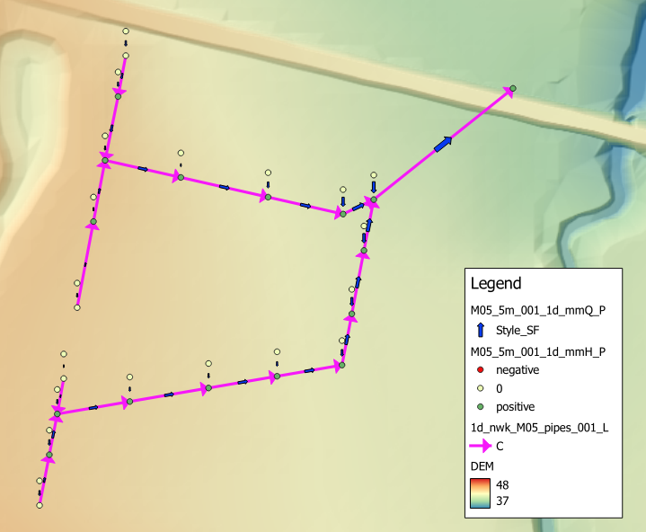
Figure 15.1: Maximum and Minimum Water Level and Flow Output

The following attributes are contained in the 1d_mmH layer:

Node: ID of the node.
Hmax: maximum water level.
Hmin: minimum water level.
tHmax: time of occurrence of the Hmax value.
tHmin: time of occurrence of the Hmin value.
dH: the largest water level drop across the channels that end at that node. Only channels that are digitised so that their downstream end is at the node are used to determine dH. Provided channels are digitised from upstream to downstream this is useful for identifying any increases in water level caused by any instabilities (thematically map the dH attribute – negative values indicate the water levels are increasing downstream). Pit channels are excluded from determining dH.

The following attributes are contained in the 1d_mmQ layer:

Channel: ID of the channel.
Qpeak: equal to the absolute maximum (positive or negative) flow. This is particularly useful for tidal reaches or where a channel has significant flows in both directions.
Qmax: maximum flow.
Qmin: minimum flow.
tQpeak: time of occurrence of the Qpeak value.
tQmax: time of occurrence of the Qmax value.
tQmin: time of occurrence of the Qmin value.
dHmax: difference in maximum water level drop through the channel. This is useful for quickly identifying large unexpected changes in flood level.
pSmax: the slope as a percentage of the water surface along the channel. This is useful for quickly identifying any troublesome behaviour along 1D networks by viewing/searching for any negative (adverse) slopes.
Style_SF: used for the automatic styling of the output. The value is a ratio based on the the channels Qmax value, and the maximum of all vMax values within the table and will range between 0 and 1.
Style_dir: angle based on the channels digitised direction.

The following attributes are contained in the 1d_mmV layer:

Channel: ID of the channel.
Vpeak: equal to the absolute maximum (positive or negative). This is particularly useful for tidal reaches or where a channel has significant flows in both directions.
Vmax: maximum velocity.
Vmin: minimum velocity.
tVpeak: time of occurrence of the Vpeak value.
tVmax: time of occurrence of the Vmax value.
tVmin: time of occurrence of the Vmin value.
Style_SF: used for the automatic styling of the arrow. The value is a ratio based on the the channels Vmax value, and the maximum of all Vmax values within the table and will range between 0 and 1.
Style_dir: angle based on the channels digitised direction.

15.2.3 ccA GIS Layer

The _ccA GIS layer contains a summary of information for culverts and bridges. It includes the following attributes:

Channel = The ID of the channel.
pFull_Max = The percentage of the peak flow area over the culvert/bridge area. If the culvert/bridge flowed full at any point during the simulation this will be 100%.
pTime_Full = The percentage of time the culvert/bridge ran full over the time the culvert/bridge ran at least 10% full.
Area_Max = The peak flow area that occurred during the simulation.
Area_Culv = The culvert/bridge flow area (when full).
Dur_Full = The time in hours the culvert/bridge was running full.
Sur_CD = Surcharge cut-off depth. Depth above pit upstream invert for a pit to be considered surcharging.
Dur_Sur = Duration of surcharge. Total duration (hrs) that the pipe is considered surcharging.
pTime_Sur = Percent time that the pipe is surcharging relative to the time the pipe is running at 100% full.
TFirst_Sur = Time of first surcharge (hrs).
Dur_10pFull = The time in hours the culvert/bridge ran 10% full or more.

The layer’s lines can be coloured and thickened according to the pFull_Max attribute (styled using the QGIS TUFLOW Plugin ‘Apply TUFLOW Styles’ Tool for .shp/.gpkg format or output directly for the .mid/.mif format). The thinner and paler the line, the smaller the pFull_Max value. The pFull_Time attribute is also useful for thematically mapping in GIS to identify culverts that are performing well, and others that are not. The example shown in Figure 15.2 illustrates the _ccA GIS layer output.

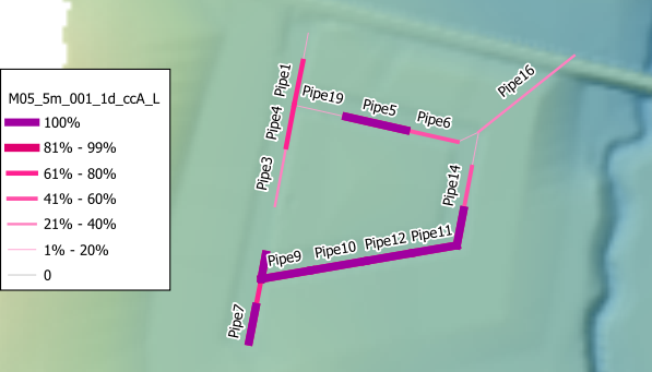
Figure 15.2: Example of the ccA GIS Layer Highlighting Culvert Performance

15.2.4 _TS GIS Layer

The 1D water levels at nodes (_1d_H.csv), and flows (_1d_Q.csv) and velocities (_1d_V.csv) in channels are output in separate .csv files. This information is also provided in the _TS GIS layer and within the .eof file (Section 14.5). Maximum and minimum values are not output to the .csv files however are contained within both the _TS GIS layer and the .eof file as well as the 1d_mmH, 1d_mmQ and 1d_mmV GIS layers (Section 15.2.2).

The _TS GIS layers contain time-series output with each layer presenting different information, as described below and in Table 15.2. In addition to the time-series data, each layer contains several attributes at the start, summarising the time-series data. These attributes are:

The maximum and minimum values;
The time in hours of the maximum and minimum values; and
The average and the average of the absolute mass error values (for the TSMB and TSMB1d2d files only).

Table 15.2: _TS GIS Layer Descriptions
GIS Layer Name	Description
_TS_L _TS_P	Contains all 1D channel (velocities and flows), 1D nodes (water levels) and 2D PO (plot output locations from 2d_po layers).
_TSF_P	Contains the flow regime flags for culverts (see Table 5.6), and other types of channels (see Table 14.2).
_TSL_P	Contains the loss / discharge coefficients for the following 1D channels: For culverts: the three values shown for each time are the inlet (entry) loss coefficient; additional loss coefficient (this value is the sum of any 1d_nwk Form_Loss (bend loss) value on the channel or an upstream pit and any manhole energy loss contribution); and outlet (exit) loss coefficient. If Structure Losses == ADJUST or the “A” flag has been specified, the entry and exit loss coeficients are adjusted loss coeficients. If there is a manhole connected to one/both ends of a culvert, the loss coefficients will be affected by any manhole energy losses, as discussed in Sections 5.10.4. For B bridges: the bridge loss coefficient adopted is shown. For BB bridges: the two values shown for each time are the bridge loss coefficient and the combined entry/exit loss coefficient. If Structure Losses == ADJUST or the “A” flag has been specified, the combined entry/exit loss coeficient is the adjusted loss coeficient. For BArch bridges: the two values shown for each time are the downstream blockage (J3) and froude number (F3) used in the ‘Afflux at Arch Bridges’ (HR Wallingford, 1988) method. If orifice flow condition is applied, the two values are the orifice flow discharge coefficient and the calibration facotor of the discharge coefficient. For advanced weirs (Section 5.7.4.3) and DF channel (Section 5.9.8.2): the flow regime is shown followed by two numbers. The first number is \(C_{f} \times C_{d}\) and the second number is \(C_{sf}\), see Equation (5.11).
_TSMB_P	Contains the mass errors at 1D nodes (refer to Section 14.7).
_TSMB1d2d_P	Contains the mass errors across 1D/2D interface linkages, ie. HX links (refer to Section 14.7).

The _TS GIS layers can be loaded into QGIS. Once loaded, they will automatically appear in the TUFLOW Viewer Results window, allowing users to view time-series data, as shown in Figure 15.3.

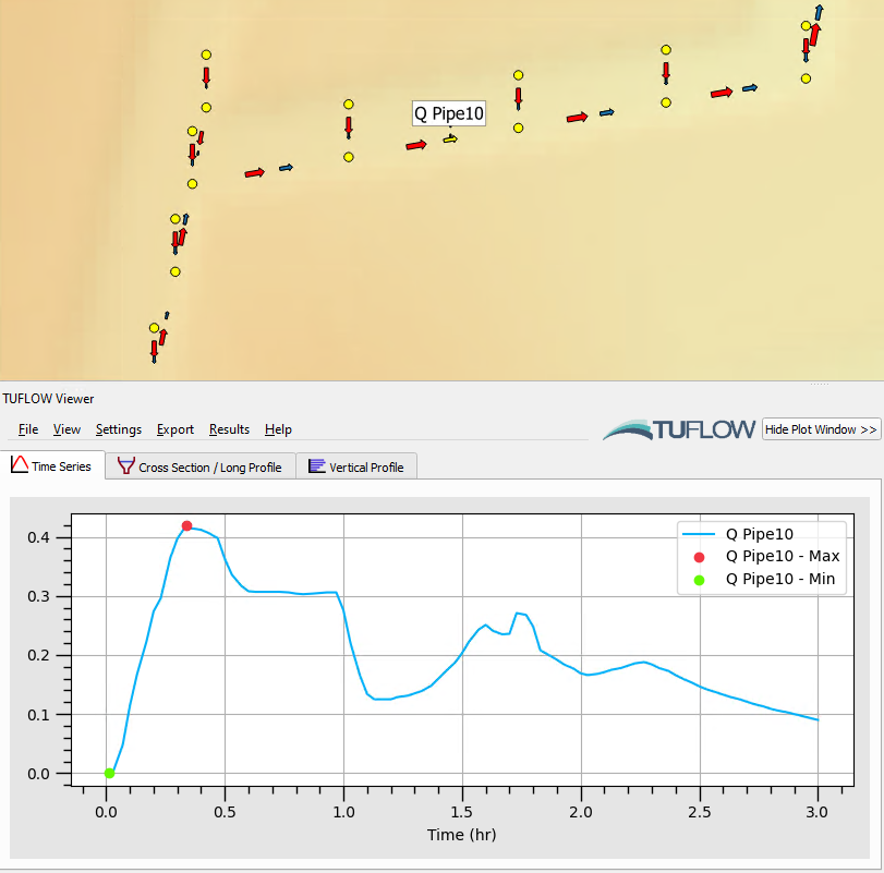
Figure 15.3: Example of the _TS Layer Flow Output

There are two ways to style the _TS layers. The first way is the default TUFLOW Styling, which displays arrows for velocity and flow, and points for water level. The second way is by using the Stability Checking Styling Tool. This tool styles the _TS layer into categories: likely unstable, possibly stable and stable, as shown in Figure 15.4. How to use this tool, and the rules applied to the categories are discussed on the TUFLOW Wiki Stability Checking Styling Tool page.

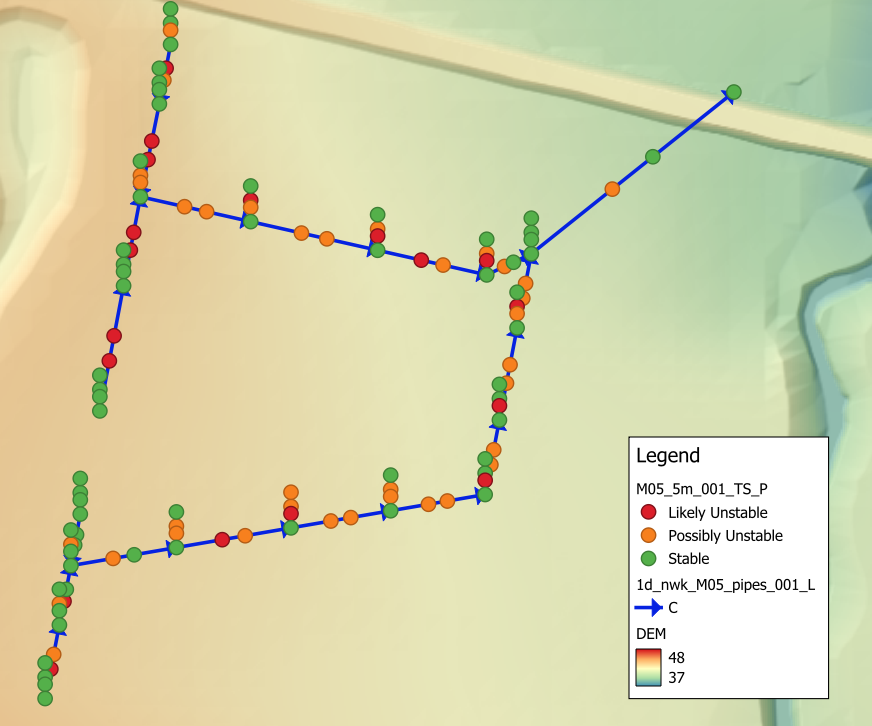
Figure 15.4: Example of the _TS Layer Stability Styling

Note that the output frequency of the time output in _TS GIS layers is automatically adjusted so that the limit of 245 output times is not exceeded (this limit is the maximum number of attributes allowed in some GIS software). For example, if based on the Time Series Output Interval setting there are 400 output times, then every second time will be written to the _TS GIS layer giving a total of 200 output times, but at least the full hydrograph is displayed!

For models that contain 1D operational structures (refer to Section 5.9), an additional file (_1d_O.csv) will be output to the “results\plot\csv” folder containing information on the operation of each structure over time. This file serves as a valuable check for the commands defined within the .toc.

15.2.5 1D Water Level Lines (WLL)

As mentioned in Section 11.2.4, 1D domain results can be output in combination with 2D domain(s) by using the 1d_wll GIS layer and the Read GIS WLL command. When WLL are used, the water level from the 1D node is interpolated into a 2D format when viewing the results (for both mesh and grid outputs). If the 1D WLLs and 2D domains overlap, the 1D results are displayed on top of the 2D results. Viewing of these 2D mesh and raster results is discussed in Section 15.3.1 and 15.3.2.

Additionally, viewing of 1D results in a 2D domain using the WLL functionality is demonstrated in TUFLOW Tutorial Module 11.