7.3 TUFLOW HPC Specific
This section describes 2D domain functionality that is unique to TUFLOW HPC.
7.3.1 Quadtree
Quadtree grid refinement functionality enables the user to vary the 2D cell resolution within a TUFLOW HPC model. Quadtree refinement allows for recursive division of square TUFLOW cells into four smaller square cells. Up to 9 levels of cell size refinement are permitted. All cells for all levels of refinement share a common orientation. Bill Syme, one of the TUFLOW author’s, discusses the benefits and implementation of Quadtree within the Future of 2D Hydraulic Modelling AWS Video. The How to Implement Quadtree video also useful. An example quadtree mesh is presented in Figure 7.26.
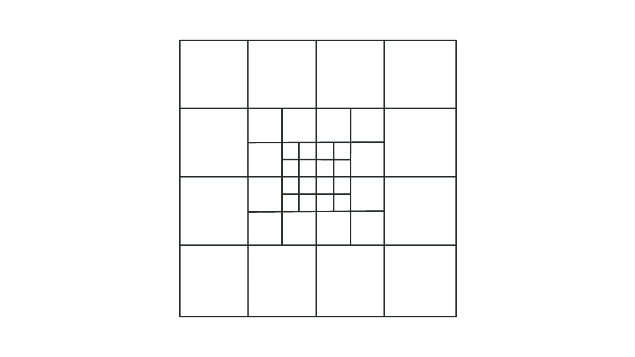
Figure 7.26: TUFLOW HPC Quadtree Grid
The Quadtree solver uses a modified version of the HPC solver. It uses an explicit finite volume solution that is 2nd order in space and 4th order in time, however there are some subtle differences between the HPC single grid and Quadtree solvers that mean they produce near identical, though not identical results if both run are over the same single grid (same cell size) grid – see Section 3.1.4 for further discussion.
The Quadtree solver uses a modified cell selection methodology for sampling datasets from line geometries, as described in Section 7.2.5.2.
TUFLOW Tutorial Module 7 provides a demonstration of quadtree. The following sections outline how to use the feature.
7.3.1.1 Quadtree .tcf Commands
To use a Quadtree grid, the solution scheme should be set to HPC and a Quadtree Control file (.qcf) specified using the command Quadtree Control File. GPU Hardware is also recommended. For example:
Note, the keyword “Single Level” can be used instead of a control file (e.g. “
The Quadtree Control File (.qcf) is described in the next section.
7.3.1.2 Quadtree Control File (.qcf) – Mandatory Commands
The Quadtree Control File (.qcf) is used to define the grid refinement areas and optionally the model location and extent for a Quadtree grid. Appendix H lists and describes the available .qcf commands.
The following commands are mandatory in a .qcf file.
If set to “AUTO” the extents of the Level 1 GIS polygon are used to define the model origin and extents. If set to “TGC”, the model is located as per the commands in the .tgc file. Note, the angle of the model is defined in the .qcf file using the Orientation Angle command below. Also, if set to “AUTO” the GIS nesting polygons must have a Level 1 polygon defined, otherwise an ERROR is generated.
The Read GIS Nesting command can be used to define polygons of grid refinement (different levels) in the 2d_qnl format file, as described in Section 7.3.1.4.
7.3.1.3 Quadtree Control File (.qcf) – Optional Commands
The following commands are optional in the Quadtree Control File:
Note: Metric (SI) units are TUFLOW’s default. To set
Base Cell Size sets the Level 1 (parent) cell size. This will be the largest cell size in the Quadtree grid. If set to a numerical value this will override the cell size command in the .tgc file. If this command is not specified or is set to “TGC”, the cell size defined in the .tgc file is used.
If set to a numerical value this defines the grid orientation angle and overrides any angle / location .tgc commands. If set to “OPTIMISE” the parent Level 1 polygon is used to optimise the angle of the grid to minimise the area of the bounding rectangle, thereby minimising temporary memory requirements during the simulation startup (the memory footprint during the simulation is not affected). As such the GIS nesting polygon must have a Level 1 polygon defined. If the command is not specified or is set to “TGC”, the orientation angle in the .tgc is used.
When pre-processing the Quadtree grid, a hidden 2D domain is used for areas of refinement to allow fast processing of geometry on a regular grid. The default approach is that each nesting level is treated as a 2D rectangular domain, and for example, with three levels of nesting the geometry control file is processed three times. To reduce initialisation memory demands it is possible to treat each GIS polygon in the 2d_qnl layer as a separate domain for the processing of geometry inputs. This is set using the optional .qcf control file command:
This allows changing to a more memory efficient approach to process each polygon in the 2d_qnl layer. However, whilst being more memory efficient during grid creation, the model startup may be slower. How the grid is processed has no effect on the speed of the hydraulic computations or the memory demand during the hydraulic calculations.
7.3.1.4 Defining Grid Refinement Polygons
A 2d_qnl (Quadtree Nesting Level) GIS layer (see Table 7.25) is used to define the location and levels of grid refinement. The 2d_qnl layers should only contain polygon / region objects, with all other GIS object types (lines, points, etc.) ignored.
The nesting level attribute must be in the range 1 to 9. A value of:
- 1: indicates that the cell size to be used for that polygon is the Level 1 or base cell size (see Base Cell Size).
- 2: indicates the cell size within the polygon would be at Level 2 (i.e. half the base cell size).
- 3: indicates the cell size within the polygon would be at Level 3 (i.e. 1/4th of the base cell size).
- 4: indicates the cell size within the polygon would be at Level 4 (i.e. 1/8th of the base cell size).
- …
- 9: so on up to a maximum of Level 9 (1/256th of the base cell size).
There should only be one Level 1 polygon defined in the 2d_qnl layer, but for all other levels there is no limit on the number of polygons. For numerical precision reasons when running single precision, the maximum nesting level of 9 or 1/256 of the base cell size has been adopted, but can be increased for double precision mode should there be a demand from users.
Note, for Z shape (2d_zsh) polygons (Section 7.2.6.2) with any merging of elevations at undefined vertices (merge polygons) which extend across multiple quadtree nested layers, it is recommended to carefully review the _zsh_zpt check file to ensure appropriate representation. CHECK/WARNING 2934 will be written in this instance.
| No. | Default GIS Attribute Name | Description | Type |
|---|---|---|---|
| 1 | Nest_Level |
The value of the quadtree nested level used for grid refinement. The nesting level attribute must be in the range 1 to 9. For example:
|
Integer |
When refining grid areas, if a refinement polygon sits within a polygon of the next higher level (e.g. a Level 3 polygon is defined within a Level 2), as per Figure 7.27, no automatic grid refining is required.
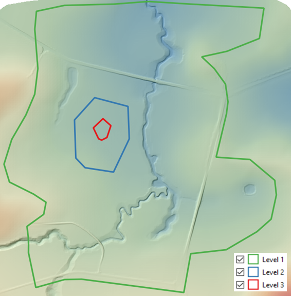
Figure 7.27: Example of Quadtree Nesting Level Polygons
However, if a nesting level polygon does not sit within a polygon of the next higher level (e.g. a Level 4 polygon is defined within a Level 1 or Level 2 polygon), intermediate areas of refinement are automatically generated by TUFLOW. For example, Figure 7.28 show the grid generated when transitioning from a Level 1 to Level 3 and a Level 1 to Level 5.
Figure 7.28: Examples of Automatic Quadtree Refinement
No Level 1 polygon is required if the model origin and extent are defined in the .tgc file. In this situation the rectangle representing the .tgc computational domain is used as the Level 1 polygon. For example, if the .qcf file includes the following commands and the only 2d_qnl polygon is Level 3 (red polygon in Figure 7.31. The grid created is based on the rectangular computational domain in the .tgc file (as shown by the thick dashed black line) with inactive cells removed from the grid to reduce memory.
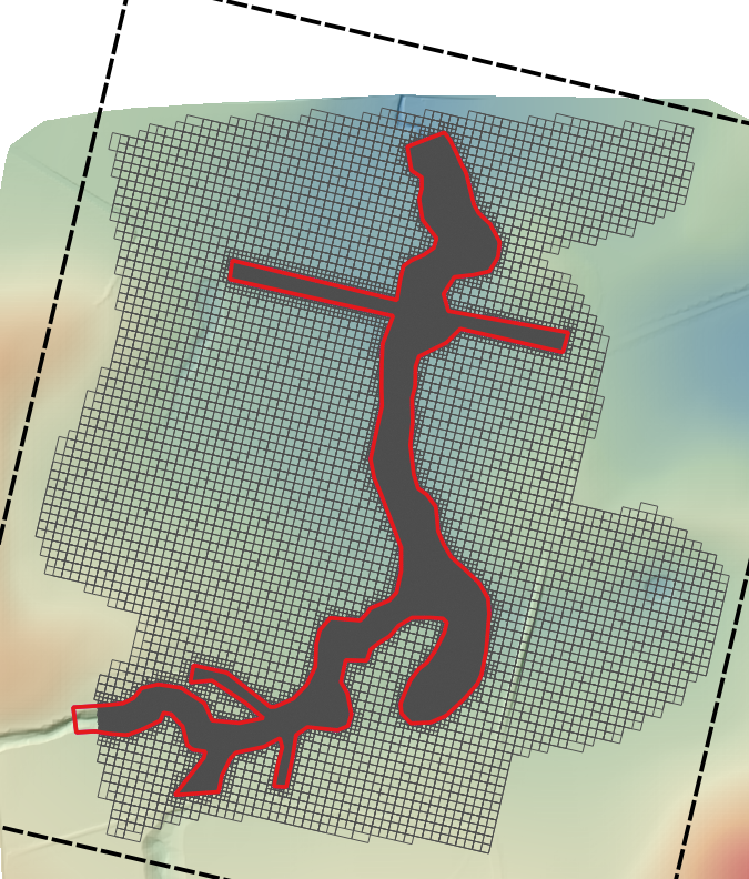
Figure 7.29: Example Showing Removal of Inactive Cells
7.3.2 HPC Turbulence
This section contains information relating to sub-grid-scale turbulence options for TUFLOW HPC.
7.3.2.1 Overview
For TUFLOW HPC, three options exist (Constant, Smagorinsky and Wu) for specifying eddy viscosity for the 2D domains to approximate the effect of sub-grid-scale turbulence. Collecutt et al. (2020) discusses the turbulence models in respect to model cell size sensitivity, resulting in the Wu approach (Section 7.3.2.4) becoming the default for TUFLOW HPC from the 2020-01 release and onwards. Discussion on the change in defaults is available in the TUFLOW Wiki HPC Turbulence FAQ page.
The Viscosity Formulation and Viscosity Coefficient commands are used to set the formulation and coefficients. Note that these commands may also be used to select the non-Newtonian module, which is discussed in Section 7.3.6 since it is not a sub-grid turbulence model.
7.3.2.2 Constant Eddy Viscosity
The Constant approach (
7.3.2.3 Smagorinsky Approach
TUFLOW’s Smagorinsky approach (
However, this approach has two known limitations:
- It assumes that all turbulent kinetic energy with length scales greater than the cell size is resolved within the velocity field. This assumption is reasonable when the 2D cell size is larger than the physical depth of the flow, but becomes incorrect when the 2D cell size is smaller than the depth of the flow – turbulence in the vertical direction contributes significantly to viscosity but is not resolved in the 2D velocity field. As a result, once the 2D cell size becomes smaller than the flow depth this approach can underpredict the viscosity, and can underpredict momentum coupling from river to flood plain.
- It assumes that the physical length scales of the sub-grid turbulence scale with the 2D cell size. This is reasonable when the 2D cell size is similar to the depth of the flow, but becomes incorrect when the 2D cell size becomes significantly larger than the depth of the flow – the bed resistance and the finite depth of the flow prevent large scale turbulence. As a result, once the 2D cell size becomes much larger than the depth of the flow, the Smagorinsky turbulence model can overpredict the viscosity, and can overpredict the momentum coupling from river to flood plain.
The result of these two limitations, is that model results display some sensitivity to the 2D cell size. The Wu formulation (Section 7.3.2.4) has proven to be more capable in its ability to provide “out of the box” calibration and reduced sensitivity of model results to 2D cell size.
Note, if the formulation is changed, the user must also reset the coefficient using the command Viscosity Coefficient.
The Smagorinsky option remains the default when using TUFLOW Classic. The default viscosity coefficients are a Smagorinsky value of 0.5 plus a constant value of 0.05 m2/s. The 0.5 Smagorinsky coefficient is dimensionless. The viscosity coefficient can be output using the Map Output Data Types command.
The hybrid Smagorinsky formulation used by TUFLOW is:
\[\begin{equation} 𝜐 = C_{c} + C_{s}A_{c}\sqrt{\left( \frac{\partial u}{\partial x} \right)^{2} + \left( \frac{\partial v}{\partial y} \right)^{2} + {\frac{1}{2}\left( \frac{|\partial u|}{\partial y} + \frac{|\partial v|}{\partial x} \right)}^{2}} \tag{7.26} \end{equation}\]
Where:
- \(u\ and\ v = \ \)Depth averaged velocity components in the X and Y directions
- \(x\ and\ y = \ \)Distance in the X and Y direction
- \(\nu = \ \)Horizontal diffusion of momentum (viscosity) coefficient, m2/s or ft2/s (if using
Units == US Customary )
- \(A_{c} = \ \)Area of Cell
- \(C_{\ c} = \ \)Constant Coefficient (default = 0.05 m2/s)
- \(C_{s} = \ \)Smagorinsky Coefficient (dimensionless, default = 0.5)
7.3.2.4 Wu Approach
The Wu approach (
Like the Smagorinsky eddy viscosity model, it is a zero-equation model whereby the eddy viscosity coefficient can be diagnostically computed from the mean depth and velocity fields. However, unlike the Smagorinsky model, where the turbulent length scale is related to cell size, the length scales used in the Wu model are related to water depth, and hence the computed eddy viscosity is not related to or dependent on cell size. This has been shown to significantly improve the cell size convergence of the results compared to the Smagorinsky model (i.e. the results are nearly independent of the cell size provided there are enough cells across the waterways to adequately define the flows).
The computed eddy viscosity is the Pythagorean sum of 3D and 2D contributions:
\[\begin{equation} \nu_{T} = \sqrt{\nu_{3D}^{2} + \nu_{2D}^{2}} \\ \upsilon_{3D} = C_{3D}U^{*}L_{m} \\ U^{*} = |U|n\frac{\sqrt{g}}{d^{\frac{1}{6}}} \\ \upsilon_{2D} = C_{2D}L_{m}^{2}|\nabla U| \\ |\nabla U| = \sqrt{\left( \frac{\partial u}{\partial x} \right)^{2} + \left( \frac{\partial v}{\partial y} \right)^{2} + \frac{1}{2}\left( \frac{\partial u}{\partial y} + \frac{\partial v}{\partial x} \right)^{2}} \tag{7.27} \end{equation}\]
Where:
- \(\nu_{T}\ \) is the final total 2D viscosity
- \(\nu_{3D}\ \)is the vertical 3D viscosity contribution
- \(\nu_{2D}\ \)is the horizontal 2D viscosity contribution
- \(C_{3D}\) coefficient for 3D viscosity contribution
- \(C_{2D}\) coefficient for 2D viscosity contribution
- \(U^{*}\) is the friction velocity (is \(\sqrt{\frac{\tau_{bed}}{\rho}}\))
- \(L_{m}\) is the turbulent length scale (is lesser of flow depth or distance to wet/dry boundary)
- \(n\) is Manning’s bed friction (see note below on treatment of high Manning’s n materials)
- \(g\) is gravity
- \(d\) is water depth
- \(|\nabla U|\) is the magnitude of the 2D velocity strain tensor
The computed viscosity \(\nu_{T}\) can be output using the Map Output Data Types command. In our testing to date, we have found \(C_{3D} = 7\) and \(C_{2D} = 0\) to yield results that agree well with benchmark tests and that are not significantly dissimilar from those of the previous Smagorinsky method with its default coefficients for situations where the depth is not significantly greater than the cell-size. The values of \(C_{3D} = 7\) and \(C_{2D} = 0\) are the default values but can be changed using the Viscosity Coefficient command. This effectively ignores the 2D component in the Wu model. Alternatively, to use only the 2D component of the model (and ignore the 3D component), we have found \(C_{3D} = 0\) and \(C_{2D} = 4\) to be a suitable starting point. As always, calibration remains an essential step. If quality calibration data is available and all Manning’s values are within industry standard ranges, then we encourage the user to adjust the coefficients as necessary to achieve calibration. We anticipate that calibration should be possible with either \(C_{2D}\) or \(C_{3D}\) in the range 1 to 7. If values outside this range are required then this may indicate other errors (eg. boundary values or schematisation, poor input data, etc). As always, sensitivity testing of changes in parameters on the model results should also be performed.
It is a common practice to represent buildings in a model as roughness (i.e. cells with high Manning’s bed friction), see discussion on modelling buildings in Section 7.2.11. As the friction velocity includes the Manning’s value, this results in a very high viscosity value at those cells. This is not unreasonable, but for TUFLOW HPC, which handles the viscosity explicitly, this can drive the timestep down to small values. We have found that limiting the Manning’s values used in the Wu 3D model to a sensible maximum (for example 0.1) makes very little difference to the model results but can vastly improve solution time. This upper limit is included as an optional third value to the Viscosity Coefficient when using the Wu approach. Note that the original high Manning’s value, as defined in the materials database, is used in the momentum equation where its primary influence is effected.
7.3.3 Sub-Grid Sampling (SGS)
Sub-grid sampling (SGS) stores elevation points sampled at a finer resolution than the 2D cell to more accurately represent the variations in terrain inside the cell, as shown in Figure 7.31. SGS functionality is introduced in Section 3.2.3. See Section 7.1.3 for a description of 2D cell control points and 7.2.4 for a description of the traditional approach to sampling datasets. Benchmark testing has shown the benefits of using SGS to be substantial, as discussed in Section 3.2.3.1.
SGS translates the high-resolution sampled elevation data into cell curve functions for its hydraulic calculations.
- The cell volume is stored as a non-linear function of elevation (i.e. a curve of cell volume versus elevation based on the wetted surface area versus depth measured from the lowest sampled elevation within the 2D cell).
- Across each cell side the flow area and flow width are calculated based on sampled elevations to produce a non-linear function of conveyance versus elevation (i.e. a curve of conveyance versus elevation. For determining the depth and width averaged velocity across each cell face the flow area is also retained as a curve of area versus elevation).
The elevation dataset sample resolution can be defined by the user. For example, using a 8m cell size and a 2m SGS Sample Target Distance the DEM is sampled at 5 points across each face. Shown in Figure 7.31 this translates to 25 elevation points being used to define the volume vs elevation relationship within the 2D cell, and 5 points along each cell side for defining the conveyance-elevation relationship of each face.
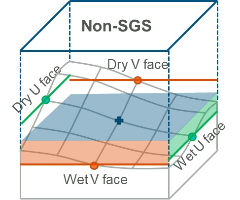
Figure 7.30: Traditional (non-SGS) Approach
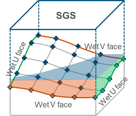
Figure 7.31: SGS Approach
The flow or conveyance of water through 2D cells is determined through a full 2D solution of the momentum equation (see Section 7.1). The bed resistance term (e.g. Manning’s equation) and the determination of the 2D velocities are controlled by the conveyance properties of each cell face. If there are considerable variations in bed topography across the cell faces, SGS will provide a significantly more accurate representation of these variations, compared to a traditional 2D cell with a single elevation value per cell face.
If the resolution of the DEM data layer is coarser or similar to the 2D cell size, the use of SGS will have little or no benefit. For example, if the DEM resolution is 2m and the cell size is 2m there is little benefit in using SGS, although a slight improvement would result as the slope of the terrain across the cell would be picked up if using SGS. In contrast, if the cell size is 20m there would be considerable benefit in using SGS as the variations in terrain across the 2D cell will be represented. TUFLOW requires an odd number of sample locations across a cell face to ensure the cell mid-face and cell corners are sampled. The number of sample locations across a cell face is referred to as the SGS Sample Frequency.
Note, if the elevation input data has a reasonable representation of the channels, Read GIS Z Shape or Read GIS Z Line “MIN, GULLY or LOWER” lines are not required, or recommended, when using SGS. Including gully lines can overestimate conveyance in these channels.
The following section will focus on implementing SGS and options regarding SGS outputs.
7.3.3.1 SGS Methodology and Commands
To implement SGS the only additional command required in the .tcf is “
By default, using this command will set:
- the SGS Approach to Method C. Prior to 2023 release the default was Method B. The default Method C is the recommended approach and older versions are considered legacy though are still provided for backward compatibility.
- the SGS Sample Frequency to sample at the minimum grid elevation resolution that can be found from grids read in to the .tgc.
7.3.3.1.1 SGS Sample Distance
To manually set the SGS distance, the recommended approach is to use the .tcf SGS Sample Target Distance command. TUFLOW requires an odd number of sample locations across a cell face, the number of sample points is calculated from Equation (7.28)
\[\begin{equation} \text{Sample Frequency} = \frac{\text{TUFLOW Cell Size}}{\text{Target Distance}} + 1 \tag{7.28} \end{equation}\]
For example, using a cell size of 10m and a sample target distance of 1m, TUFLOW will use 11 sample points along the cell face. If the target distance specified gives an even number, TUFLOW will round up to the next odd number. For example, using a cell size of 5m and a sample target distance of 1m, TUFLOW will use 7 sample points instead of 6 points along the cell face. The adopted sampling frequency is reported in the .tlf.
It is also possible to specify the SGS Sample Frequency directly instead of the target distance. When using this command with a quadtree model (see Section 7.3.1), frequencies can be set for each nested level. For example, a model with three quadtree nested levels could use
To obtain the maximum resolution, the sampling frequency can be calculated as the TUFLOW cell size divided by the DEM resolution. If this yields an even number, then it should be rounded up as per Equation (7.28). Note, there is no benefit to specify an SGS target distance smaller than the DEM resolution.
If neither the SGS Sample Target Distance or SGS Sample Frequency commands are specified, a scan of the Geometry Control File (.tgc) is performed to find the minimum raster grid resolution used in any Read Grid Zpt commands, and this is used as the sampling target distance to compute the sampling frequency. If there are no gridded elevation datasets, a default sampling frequency of 11 is used. In summary, there are four ways for the SGS Sample Frequency to be defined; in decreasing order of priority they are:
- “
SGS Sample Frequency == ” command. - “
SGS Sample Target Distance == ” command. - Target distance automatically based on the minimum grid elevation resolution in the .tgc.
- Default Sampling Frequency of 11 per face / 121 per cell.
Note: the sampling frequency per face is capped at 31 by default to avoid long pre-processing times and high memory usage. In general, a sampling frequency of between 11 and 31 is sufficient for most natural water ways or artificial structures, and users may not benefit from applying a super fine sample distance against the model cell size. However, if required, high sampling resolution is possible and the set upper limit can be increased by using the following tcf command:
Note, a hard limit of 127 per face (16,129 samples per cell) still applies.
7.3.3.1.2 SGS Topographic Updates
The approach by which topographic updates modify SGS elevations depends on the specific topographic feature. There are three types of SGS topographic update approaches:
- The topographic update layer directly modifies the SGS elevations.
- The topographic update layer modifies the cells ZC, ZU, ZV and ZH Zpts first. Then all SGS elevations within the cell are sampled from the sloping cell faces and sloping cell areas created by the modified control Zpts.
- The entire cell/face is updated based on one flat elevation value.
Not all topography update features are currently supported for SGS. Table 7.26 summarises the update approach adopted by available features and lists any unsupported features.
| Full SGS Sampling using Sample Distance | Uses ZC/ZU/ZV/ZH values | Sets Flat Cell/Face | Unsupported Features |
|---|---|---|---|
| Create TIN Zpts | Read GIS Z Shape (Breaklines) | Set Zpt | Read GIS Z HX Line |
| Read Grid Zpts | Read GIS Layered FC Shape (Breaklines) | Read GIS Variable Z Shape | Read GIS FC Shape |
| Read TIN Zpts | Read GIS Z Line | Read GIS Z Shape Route | Read GIS Zpts Modify Conveyance |
| Read GIS Z Shape (Regions) | Read GIS Zpts (Regions) |
1D Nodes with SXZ Flag
(SGS SX Z Flag Approach |
Read RowCol Zpts |
| Read GIS Layered FC Shape (Regions) |
1D Nodes with SXZ Flag
(SGS SX Z Flag Approach |
1D Pits with SXL Flag
(SGS SX Z Flag Approach |
Interpolate ZC / ZHC / ZUV / ZUVC / ZUVH |
|
1D Pits with SXL Flag
(SGS SX Z Flag Approach |
Set Code with Clean Zpt | ||
|
ZC |
The below provides a summary of SGS specific considerations for implementing 2d_zsh modifications (see Section 7.2.6.2):
- 2d_zsh polygons and TINs directly modify all SGS resolution sample points within the polygon based on the TIN triangulation. However, 2d_zsh lines modify elevations based on the cell’s control Zpts, as described in Section 7.3.3.1.3 – SGS Z Shape Line Approach. See Table 7.26.
- By default, a gradient is applied along the cell face (using the side and corner ZH, ZU and ZV Zpts) for all 2d_zsh line types. For thick and wide lines, a sloping cell area for the cell volumes (using ZC, ZU, ZV and ZH Zpts) is also applied. SGS points are sampled from these. See Section 7.3.3.1.3 – SGS Z Shape Line Approach for details.
- For partially selected cells at a 2d_zsh wide line buffer’s boundary, a sloping cell area is determined based on the cell’s modified Zpts within the buffer and the unmodified Zpts outside the buffer. All SGS sample points will be updated within the partially selected cell.
Note: It is recommended to consider alternative TIN 2d_zsh modification methods via Read GIS Z Shape 2d_zsh polygons or Create TIN Zpts to improve representation.
- For partially selected cells at a 2d_zsh wide line buffer’s boundary, a sloping cell area is determined based on the cell’s modified Zpts within the buffer and the unmodified Zpts outside the buffer. All SGS sample points will be updated within the partially selected cell.
- Use of the MIN or GULLY option is not recommended, as it can overestimate conveyance – see Section 7.3.4.
- It is strongly recommended to add MAX or RIDGE lines (see Table 7.6) for every hydraulic control (e.g. levees (artificial or natural), road/rail embankments, etc.) to reduce “leakiness” caused by SGS sampling. See Section 7.3.3.1.3 – SGS Breakline Detection Delta. This includes enforcing any crests of hydraulic controls created through a polygon or TIN 2d_zsh modification.
7.3.3.1.3 Advanced SGS Commands
As noted above, the only command required to implement SGS is “
When the SGS elevations are being processed, every cell face will store a curve of elevation versus flow width / flow area. Likewise, each cell has a curve defining the relationship of elevation versus cell volume. To make this memory efficient TUFLOW does not store information defining the specific locations within the cell or along the cell face where the low or high points in the topography occur. As a result, without breaklines, SGS will be more likely to allow “leaks” through a levee or embankment compared with running the model without SGS (see TUFLOW Wiki Quadtree and SGS FAQ for details). For example, if a 2D cell straddles a levee, SGS will sample the low elevations on either side of the levee and will flow at a lower level than if SGS was not applied and the 2D cell centre was located on top of the levee, causing the 2D cell to block flow until the levee is overtopped. Whilst the need to have breaklines is paramount, regardless of whether SGS is used, it is even more important for SGS models to accurately represent hydraulic controls such as levees (artificial or natural), road/rail embankments, fences, etc.
SGS Breakline Detection Delta is designed to identify locations where ridge lines may be required. As noted in Section 7.3.3, Read GIS Z Shape or Read GIS Z Line “MIN, GULLY or LOWER” lines are not recommended for use. See the TUFLOW Wiki Quadtree and SGS FAQ page for more details.
The SGS breakline detection check processes each 2D cell to identify the minimum water surface elevation needed for a continuous wet connection through the cell traversing between left to right and top to bottom. The maximum invert elevation of the left and right faces is subtracted from the left-right minimum water level and reports it as “uDelta”. Similarly, the top to bottom value is reported as “vDelta”. uDelta and vDelta represent the depth of water over the cell face inverts by which a natural ridge (break) line would block any flow. The maximum of uDelta and vDelta is output to the _grd_check file in the SGS_Delta_Z attribute. If either uDelta or vDelta exceeds the
This command can add significant time to the initialisation process, it is recommended to perform this check during model set up only, and to turn it off once the creation of breaklines is complete.
Figure 7.32 shows an example of where CHECK 3543 indicates where the uDelta or vDelta has exceeded the
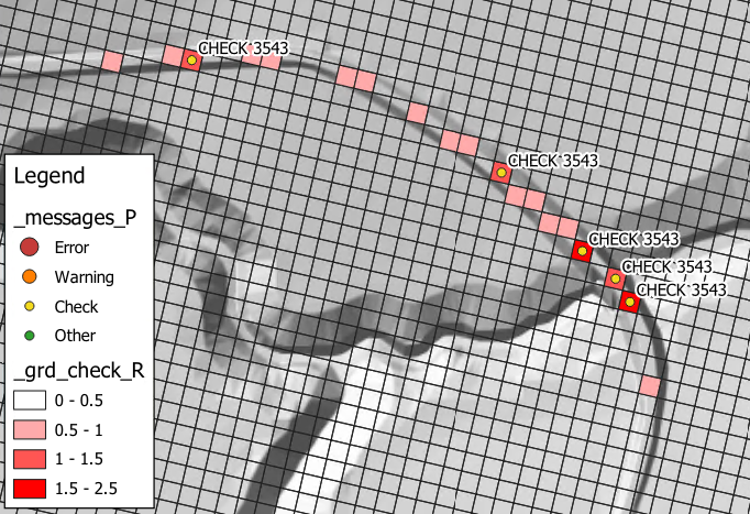
Figure 7.32: SGS Breakline Detection Delta Output
If set to Method A, cell faces modified by Read GIS Z Shape line are assumed flat (i.e. SGS is not applied and a rectangular section / flat cell is used). The default, Method B, applies a gradient along the face based on the cell corners and cell side Zpt values and for thick and wide lines uses the ZC, ZU, ZV and ZH values to apply a sloping cell area for the cell volume.
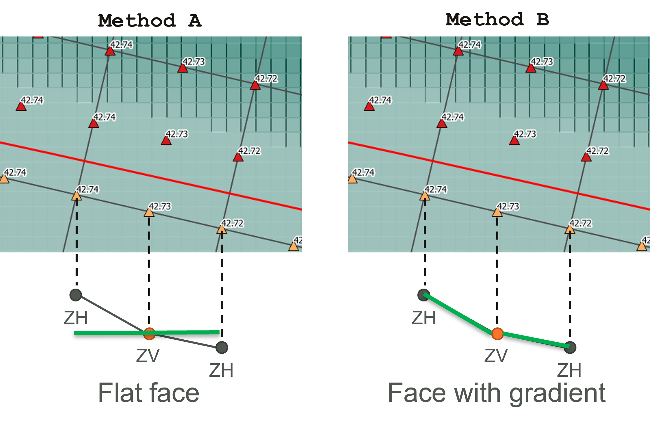
Figure 7.33: Diagram of SGS Z Shape Line Approach Options
If set to Method A, cells that are lowered by the “Z” flag on 2d_bc SX connections are assumed flat (i.e. as per the approach for no SGS). The default Method B retains the SGS information, but shifts it all to match the lowered elevation, as per Figure 7.34.
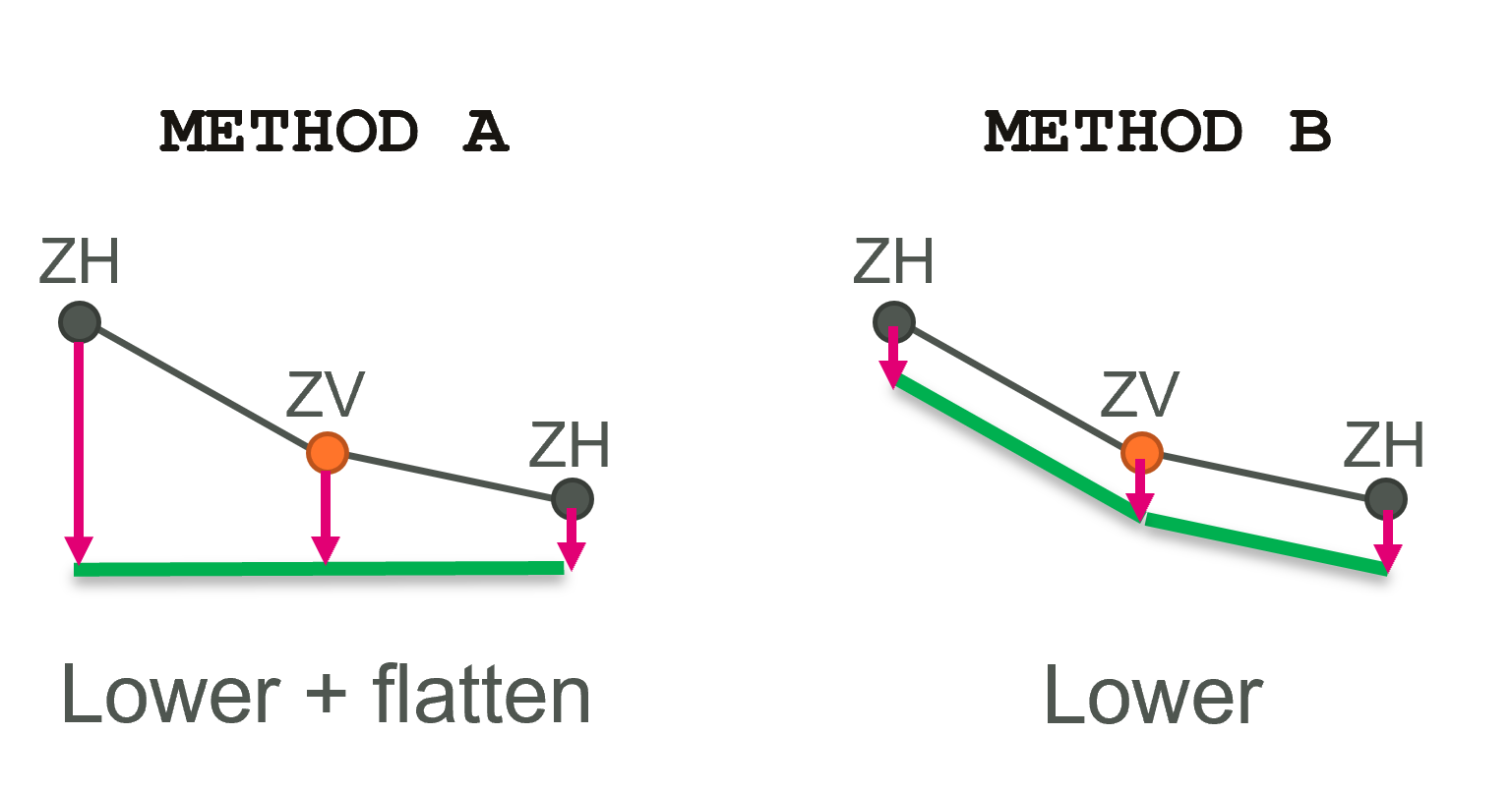
Figure 7.34: Diagram of SGS SX Z Flag Approach Options
It is possible to control the cell area used when infiltration is applied with SGS, using the SGS Infiltration Approach command. The three available options are:
- AUTO (the default): uses total area if there is a rainfall boundary and wetted area if no rainfall boundaries are present.
- TOTAL AREA: uses the whole cell area, regardless of the portion of the cell that is wet.
- WETTED AREA: uses only the wetted portion of the cell, for direct rainfall boundaries this may under predict the infiltration.
It is also possible to control the cell area used when negative rainfall is applied in conjunction with SGS, using the SGS Negative Rainfall Approach command. The two options available are:
- TOTAL AREA: uses the whole cell area, regardless of the portion of the cell that is wet.
- WETTED AREA (the default): uses only the wetted portion of the cell.
With SGS enabled, for cells that are partially wet the treatment of infiltration and direct rainfall is:
- For positive rainfall (i.e. rainfall on to the 2D cell), the volume source for each cell is the total cell area times the rainfall irrespective of whether the cell is partially wet or not.
- For negative rainfall (evaporation), the volume of evaporation is factored by the wet area fraction of the cell. That is, if the cell is only 10% wet, only one tenth of the cell’s total area contributes to the negative source term.
- For models with soil infiltration the infiltration rate is proportional to the wet area fraction of the cell. However, initial infiltration losses are based on the total area of the cell (i.e. infiltration will proceed at the maximum possible rate until the cumulative infiltration – also based on total cell area - equals the initial loss value) even if the infiltration occurs with the cell partially wet. This approach is adopted to conform with that required for direct rainfall, which assumes the rainfall is applied over the entire cell irrespective of whether the cell is partially wet or not. Likewise, soil capacity is based on the total cell area (i.e. infiltration will cease once the cumulative infiltration equals soil capacity), and the cumulative wet time for the Horton model will also increment for cells that are partially wet.
Method A (the default) assumes water is filling up from the bottom of the cell, and uses the depth above minimum cell elevation in the Manning’s bed friction calculation (see Equations (7.2) and (7.3)).
However, sheet flow conditions can occur in direct rainfall models on hill slopes, where water forms a thin layer and flows downstream. Using the depth above minimum cell elevation in such locations could underestimate bed friction. Method B checks whether SGS cells are subjected to sheet flow conditions or not, and uses cell averaged depth at the sheet flow cells to adjust the depth for the bed friction calculation.
Method B also fixes overestimation of water level gradient limiter for SGS models in cells experiencing sheet flow. Where flow in the 2D domain becomes upstream controlled, TUFLOW HPC triggers a weir flow approximation by applying a limiter to the water level gradient. This limiter can be wrongly triggered for SGS models in cells when water flows down a hill slope under sheet flow conditions. Method A (the default) calculates the gradient limiter using the same method as non-SGS models, while Method B applies an SGS specific calculation to address the issue above.
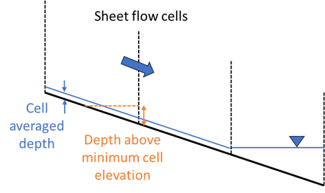
Figure 7.35: Diagram of SGS Sheet Flow Approach Options
7.3.3.2 SGS Output Options
7.3.3.2.1 Check Files
When running a model with SGS enabled there are additional attributes inserted into the _zpt check layer and an additional raster check file, the _DEM_Zmin.
If the _zpt check layer is output, with SGS turned on, the following additional attribute information is provided:
- The “Zmin” attribute for ZC points, previously called “Elevation”, now represents the minimum elevation within the cell. The “Zmin” for ZU/ZV points is the minimum along the cell face. Note, these points are still located at the centre of the cell or cell face, but the minimum value is not necessarily at this location.
- “ZExact” is the elevation at the exact location of cell centre, face mid-point, or cell corner.
- “ZAvg” is the average (mean) elevation of the sampled values.
- “ZMed” is the median elevation of the sampled values.
- The “ZMax” attribute is the maximum elevation (i.e. the elevation at which the cell area or cell face flow width is fully wet).
- “ZOut” is the elevation used for the SGS Depth Output (Section 7.3.3.2.2).
If the _DEM_Z layer is output, with SGS turned on, an additional raster output is produced, the _DEM_Z_min. The _DEM_Zmin contains a raster based on the minimum SGS elevations. When using SGS, the _DEM_Z contains a raster based on the SGS elevations used for the depth output interpolation (based on the SGS Depth Output command.)
7.3.3.2.2 Map Outputs
The following .tcf commands can be used to control the value of depth (d) map output when SGS is used.
- CELL AVERAGE (default): calculates the depth by dividing the cell volume by cell area.
- EXACT: the output depth is the water level minus the exact ZC and ZH elevations (i.e. the elevations that would be sampled exactly at the cell centre (ZC) and cell corner (ZH) locations if SGS was not applied).
- MEAN: the output depth is the water level minus the mean elevations of the cells and the cell corners from the SGS sampling. Note the MEAN depth output differs from the CELL AVERAGE depth for partially wet cells. For example, if the water level is smaller than the MEAN cell elevation, the MEAN depth output becomes negative (trimmed as zero), while the CELL AVERAGE depth (water volume / cell area) is still positive.
- MEDIAN: the output depth is the water level minus the median (50th percentile) elevation for the cells and the cell corners from the SGS sampling.
- MINIMUM: the output depth is the water level minus the minimum elevation for the cells and the cell corners from the SGS sampling (i.e. the map output shows the maximum depth within a cell / around a cell corner).
- PERCENTILE: the output depth is water level minus an elevation based on the specified set percentile. This requires a second argument, separated by vertical bar “|”, which is the percentile to use. For example, “
SGS Depth Output == Percentile | 25 ” will use the 25th percentile of the SGS elevations sampled within the cell / around the cell corner.
The elevations used for the SGS Depth Output are output in the _zpt_check file as the “ZOut” attribute, see Section 7.3.3.2.1.
Note that the water level (h) output is not affected by this command.
For the EXACT, MEAN, MEDIAN, MINIMUM, PERCENTILE approaches, the depth output is trimmed if the modelled water level is lower than the output elevations. Meanwhile, the water level output is not trimmed even if the output depth is below the output elevations, and this can produce different output extents for the water level and other outputs. For this reason, the CELL AVERAGE option is recommended for the consistency of the output extent. But if using the other options, the default trimming option can be changed using the SGS Map Extent
For the MEAN, MEDIAN, MINIMUM, PERCENTILE approaches, the corner output elevations depend on the size of the SGS sampling area around the cell corners. By default, cell corner elevations are sampled within a square that has the same size as the 2D cell. The size be manually adjusted using the SGS ZH Sample Ratio command.
By default the CELL AVERAGE depth is used to calculate the depth/velocity based map outputs, such as unit flow (q), bed shear stress (BSS), stream power (SP) and hazards, regardless of the SGS Depth Output setting. However, if desired, the depth used to calculate these map outputs can be changed using the following command:
If set to the “SGS DEPTH OUTPUT” option, the output depth specified by the SGS Depth Output command above is used. Note that the velocity (v) output is not affected by these commands.
7.3.3.2.3 High-Resolution Outputs
When using the default sub-grid sampling (SGS) approach (
High-resolution outputs and the following commands are discussed further in Section 11.2.2.3 and in Appendix A.
- HR Grid Output Cell Size: sets the map output resolution for high-resolution grid outputs.
- HR Grid Output Use Face Elevations: controls the inclusion of thin breakline cell face elevations for high-resolution outputs.
- HR Interpolation Approach: can be used to control how the cell centre / corner data is interpolated across the cell.
- HR Thin Z Line Output Adjustment: for models with thin breaklines, the presence of breaklines can be used to alter the high-resolution output interpolation.
7.3.4 2D Upstream Controlled Flow (Weirs and Supercritical Flow)
The original weir flow approximation in TUFLOW HPC was to adjust the water level gradient where flow in the 2D domain becomes upstream controlled. The 2023-03 release (and onwards) defaults to applying the full weir equation in the 2D domain along thin and thick breaklines based on the advanced weir equation (Section 5.7.4.3). However, users can revert to the original approach using the command:
Where:
- “Method A” is the pre 2023-03 method that applies the water level gradient limiter only.
- “Method B” applies the weir equation and uses the upstream water level above the weir invert as Hu, and downstream water level above the weir invert as Hd.
- “Method B Energy” is the default approach. It applies the weir equation and uses the upstream energy level above the weir invert as Hu, and downstream water level above the weir invert as Hd.
The default weir parameters (Cd, Ex, a and b) are based on the parameters used for a broad crest weir, see Table 5.16 (i.e. 0.577, 1.5, 8.55 and 0.556, respectively). The following .tcf commands can be used to change the coefficients globally.
For a thin breakline:
For a thick breakline:
A weir calibration factor can be specified globally using the Set WrF command. It can also be adjusted locally with the Read GIS WrF command, which uses a 2d_wrf GIS layer (see Table 7.27). Note WrF is not equivalent to Cf in the advanced weir equation. To be consistent with TUFLOW Classic, the weir equation is divided by WrF. This means a WrF of 1.0 represents no adjustment, while a factor greater than one will decrease the flow efficiency. The default value of WrF is 1.0.
Models using the Set WrF and Read GIS WrF functionality are provided in the 2D Structures Example Model Dataset on the TUFLOW Wiki.
| No. | Default GIS Attribute Name | Description | Type |
|---|---|---|---|
| 1 | WrF | The calibration factor used to adjust the weir equation. | Float |
7.3.5 Infiltration and Groundwater Flow
This section contains information relating to soil infiltration and groundwater flow options for TUFLOW HPC.
7.3.5.1 Infiltration
7.3.5.1.1 SCS Curve Number (SCS)
The SCS method, added in the 2025 release, uses a “curve number” (USDA, 1986) (ranging from 100 for impervious rock down to approximately 30 for deep porous soils) to define the maximum infiltration that can soak into the ground. An initial loss for the soil can be defined, typically as a fraction (termed the “initial abstraction ratio”) of the maximum infiltration. The initial loss is not considered an extra loss - the remaining soil capacity after the initial loss is filled is equal to total soil capacity (as defined in Equation (7.29)) less the initial loss. The SCS method is only available in the HPC solver - it is not available in Classic. For the soil infiltration methods supported by both Classic and HPC, see Section 7.2.8.1.
SCS infiltration differs from the alternative methods (e.g. Green-Ampt, Horton and ILCL - see Section 7.2.8.1) in the following ways:
- The maximum infiltration and the rate of infiltration are both defined by the curve number, and the initial loss by the abstraction ratio. As a result the soil capacity cannot be defined independently of the soil type, and similarly, initial water content of the soil cannot be defined independently of the soil type. Reading soil depth, porosity, and initial moisture as spatial layers are all disallowed with this method, and SCS soil types cannot be used in conjunction with any of the other soil types within the same model.
- The infiltration is defined as a fraction of the applied rainfall, which is dependent only on the curve number and the cumulative rainfall at the location in question. Infiltration does not occur if there is no rain, and the amount that occurs is defined as a fraction of the rainfall, regardless of whether or not the soil has surface water over it. The SCS method is really a rainfall loss method defined according to soil type, rather rather than physics-based infiltration.
- The SCS method is a rainfall loss method, and it can only be used with single layer soil files with groundwater depth unspecified, i.e. interflow (Section 7.3.5.2.2) is not allowed. The SCS method is not recommended for continuous simulations especially when sub surface flows may be of concern.
The parameters used in the tsoilf by the SCS method are shown in Table 7.28.
The maximum infiltration is defined (in inches) as
\[\begin{equation} S = \frac{1000 - 10C_N}{C_N} \tag{7.29} \end{equation}\]
Where:
- \(S\) is the maximum infiltration in inches (which is converted for models in SI units)
- \(C_N\) is the curve number
The initial loss is defined as a fraction of the maximum infiltration:
\[\begin{equation} IL = I_a S \tag{7.30} \end{equation}\]
Where:
- \(IL\) is the initial loss
- \(I_a\) is the “initial abstraction ratio”
For the duration where the cumulative rainfall is less than the initial loss, the cumulative infiltration must match the cumulative rainfall. After this time, the cumulative infiltration is defined as a fraction of the cumulative rainfall according to:
\[\begin{equation} CI = RFC - \frac{\left(RFC - IL\right)^2}{RFC + S - IL} \tag{7.31} \end{equation}\]
Where:
- \(CI\) is the cumulative infiltration
- \(RFC\) is the cumulative rainfall
Once the cumulative infiltration matches the maximum, \(S\), no further infiltration occurs. This occurs at a cumulative rainfall of
\[\begin{equation} RFC_s = S\left(\frac{1 - I_a + {I_a}^2}{I_a}\right) \tag{7.32} \end{equation}\]
This process is shown in Figure 7.36 for SCS curve number 50 with initial abstraction ratio 0.2. In this example the maximum infiltration, \(S\), is 10 inches, and is reached at 42 inches cumulation rainfall (marked as \(RFC_S\)).
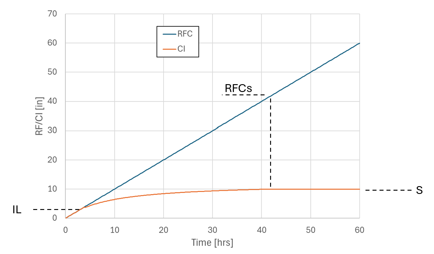
Figure 7.36: SCS Infiltration for Curve Number 50, Ia = 0.2
The instantaneous infiltration rate, during the period \(IL < RFC < RFC_s\), can then be found to be:
\[\begin{equation} IR = \left(\frac{S}{S-IL+RFC}\right)^2 RF \tag{7.33} \end{equation}\]
Where:
- \(IR\) is the current infiltration rate
- \(RF\) is the current rainfall rate
For the SCS method, the infiltration rate is based on the rainfall as applied at ground level, i.e. after the material based initial loss and continuing losses have been applied. It is worth considering that the SCS method allows for an instantaneous absorption of rain up to the initial loss (initial abstraction ratio times maximum infiltration). In this case, any materials based initial loss and continuing loss should be thought of as interception losses only. With forested areas these may be large enough that they should be included, but in open grasslands they are probably insignificant. The infiltration losses are then also reduced according to the material fraction impervious, which effectively means that:
- The soils based initial loss as defined by the initial abstraction ratio is reduced by the material fraction impervious, and
- The total loss (i.e. equivalent to soil capacity) is also reduced by the material fraction impervious. When using sub-grid sampling, the wet area fraction method selected is not used as the losses apply to rainfall, not ponded water.
7.3.5.2 Groundwater Flow
From the 2023-03 release and onwards, horizontal flow (advection) of water (Section 7.3.5.2.1) and multiple vertical groundwater layers (Section 7.3.5.2.2) when using TUFLOW HPC are supported. This groundwater flow feature is designed to model unconfined subsurface flow movement, including the saturated groundwater flow within unconfined aquifer and the variably saturated flow in vadose zone.
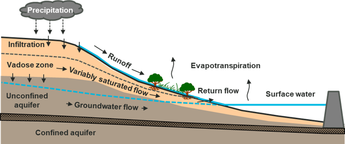
Figure 7.37: Illustration of groundwater flow movement
Up to 10 vertical layers are supported, each with horizontal advection within the layer possible, and vertical fluid movement between groundwater soil layers. Movement of water within the ground in the real world is complex. The functionality introduced in the 2023-03 release is not intended to replace detailed groundwater modelling, but provides a functional mechanism by which:
- Catchment response for 2D direct rainfall (“rain on grid”) models can be better calibrated to available river flow data.
- Long-term catchment models can be constructed that offer some prediction of stream-flows long after rainfall events.
- The accuracy of real-time flood forecasts can be improved by taking into account the drying and draining of catchments that has occurred since the last rainfall event.
- Groundwater seepage can cause inundation, such as seepage under a levee bank through a porous layer (e.g., old gravel river course), resulting in flooding on the protected side of the levee.
The basic groundwater modelling approach is conceptualised by dividing the ground into vertical layers, each with a defined thickness (alternatively a z elevation for the bottom of each layer), soil type, and cumulative infiltration of water within the layer. The cumulative infiltration, combined with the porosity defined by the soil type, allows a theoretical “groundwater elevation” (also known as a “water table”) to be computed within the layer. Figure 7.38 illustrates the soil layers in adjoining cells with convective and advective fluxes.
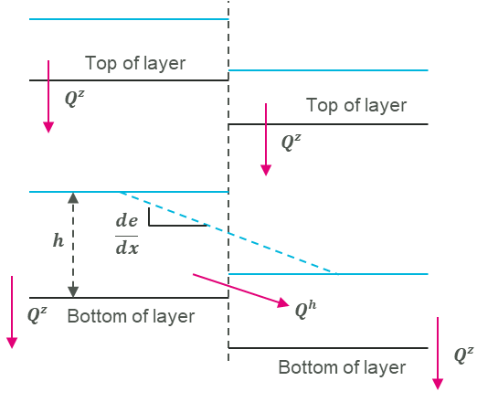
Figure 7.38: Illustration of soil layers and flows in adjoining cells
The horizontal movement of water, \(Q^{h}\), is governed by the horizontal hydraulic conductivity value set in the tsoilf file (see Table 7.28). All groundwater layers allow for horizontal advection of the water within the layer. Horizontal advection is disabled if all horizontal hydraulic conductivities are set to zero (which is the default if they are not specified). An example of a model using horizontal hydraulic conductivity, is provided in the TUFLOW Example Model Dataset.
The vertical flow of water, \(Q^{z}\), from the surface water layer into the first (or top) groundwater layer is governed by the soil infiltration model. The infiltration into the top soil can use any of the Green-Ampt (GA), Horton (HO) and Initial/Continuing Loss (IlCL) infiltration methods, as listed in Table 7.28. For layers below the top vertical soil layer then the Convective (CO) type must be used, see Section 7.3.5.2.2. An example of a model using two vertical soil layers (i.e. the “CO” type), is provided in the TUFLOW Example Model Dataset.
The cumulative infiltration data and the vertical movement of water are stored and computed at cell centres. As such, all soil data and groundwater layer geometry is sampled from the GIS / Grid layers at cell centres. Likewise the material “fraction impervious” data is sampled at cell centres (unlike the mannings values which are sampled at face centres). For the horizontal advection calculation, which is performed at cell faces, the horizontal hydraulic conductivity used is the average of the cell centre values for the adjoining cells.
7.3.5.2.1 Horizontal Advection
For all layers, the horizontal advection of water from one cell to the next, \(Q^{h}\), is computed using the horizontal hydraulic conductivity of the soil and the horizontal gradient of a variable called the “groundwater pressure level”:
\[\begin{equation} Q^{h} = - k_{h}hp\frac{de}{dx}dy \tag{7.34} \end{equation}\]
Where:
- \(k_{h}\) is the horizontal hydraulic conductivity of the soil (average of the adjoining cells used)
- \(h\) is the groundwater elevation less the layer bottom elevation
- \(p\) is the soil porosity
- \(\frac{de}{dx}\) is the gradient of the “groundwater pressure level”
- \(dy\) is the width of the face
Note, the soil porosity is often NOT included in the standard Darcy’s law equation, while the groundwater horizontal flux in TUFLOW is factored by the soil porosity. The 2025.1 release introduced a new command to turn porosity off in the horizontal flux calculation:
Note, if advection of groundwater is not required, then the advection calculation may be disabled by setting \(k_{h}\) to zero for all soils. This is the default behaviour if \(k_{h}\) is not specified in the soil parameters.
For cells that are “unsaturated” the “groundwater pressure level” is exactly the groundwater elevation within that layer. For cells that are fully saturated, the groundwater pressure level is that of the cell in the next layer above (or the water surface elevation when considering the topmost groundwater layer). For cells that are “nearly saturated” the groundwater pressure level is transitioned between these two options. The threshold at which the transition begins is called the “groundwater blending threshold”, \(\phi\).
\[\begin{equation} \xi = \frac{\frac{h_{i}}{dz} - \phi}{(1 - \phi)} \\ e_{i} = (1 - \xi)\left( z_{i} + h_{i} \right) + \xi e_{i - 1} \\ e_{0} = {WSE}_{surface} \tag{7.35} \end{equation}\]
Where:
- \(h_{i}\) is the depth of groundwater in the cell
- \(dz\) is the vertical thickness of the layer
- \(z_{i}\) is the layer bottom elevation
- \(e_{i - 1}\) is the groundwater pressure level for the layer above (or surface layer)
- \(e_{i}\) is the resulting groundwater pressure level for this layer
The layer ordering is such that the surface water is layer “0”, the highest groundwater layer is “1”, and any subsequent groundwater layers range from 2 to N (i.e. from top to bottom).
The groundwater blending threshold, \(\phi\), defaults to a value of 0.9 but can be overridden by the user in the .tcf using the command:
If the sum of flows into a layer cell causes it to exceed its soil capacity, the excess is pushed upwards to the next layer. If this happens for the top-most groundwater layer, the excess is pushed into the surface water as “return flow”. This is to be expected in the creek beds but may also happen at the bottom of steep hills where the slope transitions from steep to shallow.
7.3.5.2.2 Convective Flow Layers (CO)
For layers below the top groundwater layer, the vertical flow of water, \(Q^{z}\), is computed using a “convective” hydraulic conductivity (effectively the same concept as continuing loss):
\[\begin{equation} Q^{z} = \ - kdxdy \tag{7.36} \end{equation}\]
Where:
- \(Q^{z}\) is the convective vertical flux
- \(k\) is the convective hydraulic conductivity
- \(dxdy\) is the cell area
Note that \(Q^{z}\) is limited to the available cumulative infiltration stored in the groundwater layer above, and also limited to the remaining capacity of the groundwater layer below.
7.3.5.2.3 Unsaturated Groundwater Flow
The 2025.1 release implemented new features to adjust groundwater flux based on the saturation of soil layers. This enhancement is designed to simulate variably saturated flow (VSF) through vadose zones.
A simple adjustment based on the power function of the relative saturation can be applied to both the vertical flux and the horizontal flux:
\[\begin{equation} Q^{h} = - k_{h}h\frac{de}{dx}dyS_{e}^{Ex_{h}} \tag{7.37} \end{equation}\]
\[\begin{equation} Q^{z} = \ - kdxdyS_{e}^{Ex_{v}} \tag{7.38} \end{equation}\]
Where:
- \(S_{e}\) is the relative saturation
- \(Ex_{h}\) and \(Ex_{v}\) are the exponents of the power functions applied to the vertical flux and the horizontal flux
The relative saturation \(S_{e}\) is calculated as:
\[\begin{equation} S_{e} = \frac{\theta(t)-\theta_{r}}{\theta_{s}-\theta_{r}} \tag{7.39} \end{equation}\]
Where:
- \(\theta(t)\) is the simulated water content (fraction)
- \(\theta_{r}\) is the residual water content (fraction)
- \(\theta_{s}\) is the saturated water content (fraction)
The residual and saturated water contents (\(\theta_{r}\) and \(\theta_{s}\)) must be specified for each soil type in .tsoilf file (Table 7.28). The exponents can be specified globally by including a second argument in the following two commands:
The default values of \(Ex_{h}\) and \(Ex_{v}\) are both zero (0), i.e. the groundwater fluxes are not adjusted based on \(S_{e}\).
Note, when the vertical exponent is zero, TUFLOW ‘lumps’ soil water at the bottom of each soil layer. This means water infiltrated from the layer above can instantly move to the next layer in the next timestep, which may cause the soil water to reach the bottom layer before filling up the layers above. This simple power function was found to be effective to ‘delay’ the vertical infiltration. The optimal value for \(Ex_{v}\) depends on the layer thickness. For models that specify one or two layer(s) for the root zone (0~1m deep), an \(Ex_{v}\) value of 2 was found to produce the best results in benchmarking tests, however, calibration or sensitivity testing is recommended.
The 2025.1 release also implemented a soil moisture dependent function for the horizontal flux based on (Van Genuchten, 1980).
With this option, the horizontal hydraulic conductivity is adjusted based on the following equation:
\[\begin{equation} k_{h}(S_{e}) = k_{h}S_{e}^{L}\{1-[1-S_{e}^{n/(n-1)}]^{1-1/n}\}^{2} \tag{7.40} \end{equation}\]
Where:
- \(S_{e}\) is the relative saturation (see Equation (7.39))
- \(n\) and \(L\) are the model parameters
Note, strictly speaking, groundwater pressure level \(e\) used to calculate the pressure gradient (\(\frac{de}{dx}\)) needs to be adjusted based on the water retention curve:
\[\begin{equation} S_{e} = [1+(\alpha e)^{n}]^{1/n-1} \tag{7.41} \end{equation}\]
Where:
- \(\alpha\) is the model parameter (\(m^{-1}\))
The model parameters \(\alpha\), \(n\) and \(L\) can be specified for each soil type in .tsoilf file (Table 7.28). The recommended model parameters for different soil classes can be found from Rosetta’s technical documentation (Schaap, 2002).
Note, when
7.3.5.2.4 Implementation
Although the theory appears complex, the implementation of groundwater within the TUFLOW model files is straight forward. The essential steps are:
- Read a soils (.tsoilf) data file from within the .tcf (see Section 7.3.5.3).
- Define the soil types in the .tgc (see Section 7.3.5.2.5).
- Define the soil layer thickness in the .tgc (see Section 7.3.5.2.5).
- Specify locations of groundwater boundaries in the .tbc (see Section 8.4.1.2).
- Specify initial water levels within the soil layers (optional) (see Section 8.8.2).
- Add any additional output data types in the .tcf. For example:
- Map Output Data Types (see Section 11.2.3): dGW, GWd, GWh, GWm, GWq, GWv in Table 11.4, or
- Time series plot output data types (see Section 11.3): GWd, GWh, GWm, GWq, GWqa, GWqu, GWqv, GWVol in Table 11.9.
7.3.5.2.5 Soil Type
Setting the soil type for the groundwater layers activates the given layer. The Green-Ampt, Horton and Initial/Continuing Loss infiltration methods can be used for Layer 1. Any layers beneath Layer 1 (e.g. Layer 2, Layer 3) must be the Convective Type. For example, setting the soil type for layers 1 and 2 will activate 2 vertical groundwater layers:
Multiple layers can be set simultaneously (the below will activate 3 interflow layers):
This method also works for read GIS and Grid commands:
A maximum of 10 vertical layers is permitted and a soil ID should be assigned for each active layer. For example, if groundwater layer 2 is active, then soil IDs for layer 1 should be assigned. Note, if the layer number is not specified in a .tgc command (e.g. Set Soil), it is assumed to be layer 1.
7.3.5.2.6 Soil Thickness
The depth (thickness) of each vertical interflow layer can be set using the following commands:
If the soil layer thickness or base elevation is not set for a given layer, it is assumed to be infinite. The soil thickness sets the layer depth from the layer above and soil base elevation sets the absolute elevation of the bottom of the layer. If both methods are specified for a given grid cell, the highest of the two will be adopted. The input units should be in metres or feet (if using
7.3.5.2.7 Drying of Top Groundwater Layer
Evaporation is typically implemented with a global negative rainfall. Prior to the 2023-03 release this would only remove water in wet cells until they dry. It would not draw from the cumulative infiltration layer. The 2023-03 release and onwards allows for negative rainfall to draw from the topmost groundwater layer under surface layer cells that are dry, thus mimicking evapotranspiration. Currently onlyone approach is implemented, called “factor”, which applies the defined negative rainfall, though at a (globally) factored rate. To select this approach use the Soil Negative Rainfall Approach .tcf command.
The default approach is to not apply any negative rainfall to the topmost groundwater layer. If the “factor” method is selected, then the factor can be set using the Soil Negative Rainfall Factor .tcf command. The default factor is 1, meaning that the full value of the negative rainfall is applied. If the topmost groundwater layer is dry, then no negative rainfall is applied, and the approach does not look any further than the topmost layer. No water is drawn from subsequent ground water layers.
7.3.5.3 HPC Soils File (.tsoilf)
The .tsoilf is the same file mentioned in Section 7.2.8.2. However, when using TUFLOW HPC there are additional parameters available which can be used to enable horizontal advection, as well as two additional soil types: convective (CO) and SCS. These additional parameters are bold in Table 7.28.
| Column No. | No Intriltration | Green-Ampt | Green-Ampt | Horton | Initial/Continuing Loss | SCS Curve Number | Convective |
|---|---|---|---|---|---|---|---|
| 1 | Soil ID | Soil ID | Soil ID | Soil ID | Soil ID | Soil ID | Soil ID |
| 2 | NONE | GA | GA | HO | ILCL | SCS | CO |
| 3 | USDA Soil Type (see Table 7.14) (mandatory) | Suction (mm or inches) (mandatory) | Initial Loss (mm or inches) (mandatory) | Initial Loss (mm or inches) (mandatory) | Curve Number (see USDA (1986)) (mandatory) | Vertical Hydraulic Conductivity (mm/h or in/h) (mandatory) | |
| 4 | Initial Moisture (Fraction) (optional) | Hydraulic Conductivity (mm/h or in/h) (mandatory) | Initial Loss Rate (\(f_0\)) (mm/h or in/h) (mandatory) | Continuing Loss (mm/h or in/h) (mandatory) | Initial Abstraction Ratio (Fraction) (mandatory) | Porosity (Fraction) (mandatory) | |
| 5 | Max Ponding Depth (m or ft) (optional) | Porosity (Fraction) (mandatory) | Final Loss Rate (\(f_c\)) (mm/h or in/h) (mandatory) | Porosity (Fraction) (optional) | Residual Water Content (-) (optional) | Initial Moisture (Fraction) (optional) | |
| 6 | Horizontal Hydraulic Conductivity (mm/h or in/h) (optional) | Initial Moisture (Fraction) (optional) | Exponential Decay Rate (k) (\(h^{-1}\)) (mandatory) | Initial Moisture (Fraction) (optional) | Saturated Water Content (-) (optional) | Horizontal Hydraulic Conductivity (mm/h or in/h) (optional) | |
| 7 | Residual Water Content (-) (optional) | Max Ponding Depth (m or ft) (optional) | Porosity (Fraction) (optional) | Horizontal Hydraulic Conductivity (mm/h or in/h) (optional) | Parameter α (\(m^{-1}\)) (optional) | Residual Water Content (-) (optional) | |
| 8 | Saturated Water Content (-) (optional) | Horizontal Hydraulic Conductivity (mm/h or in/h) (optional) | Initial Moisture (Fraction) (optional) | Residual Water Content (-) (optional) | Parameter n (-) (optional) | Saturated Water Content (-) (optional) | |
| 9 | Parameter α (\(m^{-1}\)) (optional) | Residual Water Content (-) (optional) | Horizontal Hydraulic Conductivity (mm/h or in/h) (optional) | Saturated Water Content (-) (optional) | Parameter L (-) (optional) | Parameter α (\(m^{-1}\)) (optional) | |
| Parameter n (-) (optional) | Saturated Water Content (-) (optional) | Residual Water Content (-) (optional) | Parameter α (\(m^{-1}\)) (optional) | Parameter n (-) (optional) | |||
| Parameter L (-) (optional) | Parameter α (\(m^{-1}\)) (optional) | Saturated Water Content (-) (optional) | Parameter n (-) (optional) | Parameter L (-) (optional) | |||
| Parameter n (-) (optional) | Parameter α (\(m^{-1}\)) (optional) | Parameter L (-) (optional) | |||||
| Parameter L (-) (optional) | Parameter n (-) (optional) | ||||||
| Parameter L (-) (optional) |
7.3.6 Non-Newtonian Flow
TUFLOW HPC supports modelling of non-Newtonian fluids. The non-Newtonian flow theory, and an example of its use in TUFLOW is discussed in the Tsunami and Dam Failure and non-Newtonian Modelling AWS Webinar. This feature was introduced in the 2020-01 release. It is not supported in TUFLOW Classic. High-fidelity modelling of non-Newtonian fluids is complex and 3D in nature. However, with some assumptions, it is possible to model non-Newtonian fluids reasonably well in 2D. The assumptions are:
- The 2D (horizontal) viscosity can be represented as a summation of laminar (derivative of non-Newtonian shear stress model) and turbulent (from Wu eddy viscosity model) contributions.
- Acceleration effects are small and the laminar fluid shear stress is linear with depth.
- The bed shear stress can be represented as a summation of laminar (from non-Newtonian shear stress model) and turbulent (from Manning’s equation) contributions.
The laminar fluid shear stress (for flow that is shearing), is assumed to follow the Hershel-Bulkley power law model:
\[\begin{equation} \tau = \tau_{0} + k{\dot{\gamma}}^{n} \tag{7.42} \end{equation}\]
Where:
- \(\tau_{0}\) = Yield shear stress of the fluid.
- \(k\) = Viscosity parameter (units Pa.sn)
- \(\dot{\gamma}\) = Shear strain rate of the fluid
- \(n\) = Power law exponent (1 = Newtonian, <1 is shear thinning, >1 is shear thickening)
For flows where the bed shear stress exceeds the yield stress, a ‘plug flow’ velocity profile is computed, as shown in Figure 7.39. For flows where the bed shear stress does not exceed the yield stress, the fluid is considered locked to the bed and does not flow. Within TUFLOW HPC, at the start of each timestep, a bed stress is calculated for each cell such that the predicted velocity profile (for the given bed shear stress) has a depth averaged mean velocity that matches the current model velocity.
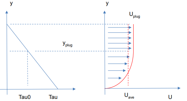
Figure 7.39: Non-Newtonian Shear Stress and Velocity Profile
Note that for fluids with a low viscosity parameter, or for deep and/or faster flows, the bed friction that would arise through the use of Manning’s equation (which is based on turbulent water flow) can be equal to or greater than that from the Hershel-Bulkley equation. In this situation the mathematics is stating that the non-Newtonian flow is likely to be turbulent and behaving more like water, and the bed shear stress as computed by the Hershel-Bulkley powerlaw model is likely to be lower than what is occurring in reality. To account for this transition in a simple manner, the actual bed friction used is the sum of both non-Newtonian and Manning’s contributions (note the n in the final term on the righthand side of the following equation is Manning’s n, not the Hershel-Bulkley power law exponent):
\[\begin{equation} \tau = \tau_{0} + k{\dot{\gamma}}^{n} + \frac{\rho gn^{2}|U|^{2}}{d^{\frac{1}{3}}} \tag{7.43} \end{equation}\]
This provides a very stable and smooth transition from non-Newtonian bed shear stress to turbulent water-like bed shear stress as and when needed. The total shear stress is then utilised in the momentum equation to evolve the flow velocity. The momentum equation also considers the possibility that the fluid yield stress is sufficient to hold the fluid against the net momentum flux, in which case the fluid velocity is zeroed.
For the computation of 2D shear stresses, the yield shear stress is not used and the fluid is allowed to continue shearing down to low shear strain rates and correspondingly low shear stresses. The effective Non-Newtonian 2D viscosity is computed using the derivative of the Hershel-Bulkley equation:
\[\begin{equation} \mu_{2D} = kn\left| \dot{\gamma} \right|^{n - 1}\\ \left| \dot{\gamma} \right| = \max\left( \frac{2|U|}{d},\sqrt{\left( \frac{du}{dx} \right)^{2} + \left( \frac{dv}{dy} \right)^{2} + \frac{1}{2}\left( \frac{du}{dy} + \frac{dv}{dx} \right)^{2}} \right) \tag{7.44} \end{equation}\]
Where:
- \(\left| \dot{\gamma} \right|\) = Magnitude of shear strain rate
Since the \(n - 1\) exponent can cause the viscosity to diverge to infinity at low strain rates for shear thinning fluids, it necessary to bound the resulting viscosity to a user defined upper limit, \(\mu_{high}\). For completeness a user defined lower limit, \(\mu_{low}\), is also applied.
Finally, for deeper and high velocity flows it is possible that the effective 2D viscosity of turbulent water, as computed by the Wu turbulence model, is greater than the value computed from the Hershel-Bulkey powerlaw model. Again, in this situation the mathematics is stating the non-Newtonian flow is likely to be turbulent and behaving more like water. To account for this transition the actual 2D viscosity used is the sum of both non-Newtonian and Wu turbulence model contributions:
\[\begin{equation} \nu_{T} = \frac{\mu_{2D}}{\rho} + 7U^{*}d \tag{7.45} \end{equation}\]
Where:
- \(U^{*}\) = Friction velocity = \(\frac{\sqrt{g}\ n|U|}{d^{\frac{1}{6}}}\)
This provides a very stable and smooth transition from non-Newtonian 2D viscosity to turbulent water-2D viscosity as and when needed. The value of 7 is the default Wu viscosity parameter and is not user-definable for the non-Newtonian module.
7.3.6.1 Implementation
The non-Newtonian flow model is invoked with the Viscosity Formulation command in the .tcf. If invoked there are no default values for the required coefficients (\(k\), \(n\), \(\mu_{low}\), \(\mu_{high}\), \(\tau_{0}\)). These must be supplied wit the Viscosity Coefficient command, where:
- \(k\): viscosity coefficient (Pa.s^n)
- \(n\): shear thickening exponent, must be non zero and positive (shear thinning fluids exhibit \(n\) < 1, shear thickening \(n\) > 1, and Newtonian fluids \(n\) = 1)
- \(\mu_{low}\): lower viscosity limit (Pa.s)
- \(\mu_{high}\): higher viscosity limit (Pa.s)
- \(\tau_{0}\): shear yield stress (Pa)
A step-by-step example of how to set up a non-Newtonian model is provided in TUFLOW Tutorial Module 5 on the TUFLOW Wiki. Additionally, an example model is provided in the Non-Newtonian Example Model Dataset on the TUFLOW Wiki.
Note: In TUFLOW HPC the 2D momentum diffusion is handled explicitly and can drive the model timestep to small values when the viscosity becomes large. For shear thinning models, it is important to define an upper limit, \(\mu_{high}\), that is only as large as necessary. We suggest starting with 1,000 Pa.s and adjusting lower if the model is being strongly controlled by the diffusion control number (Nd). Sensitivity testing should be done to test whether the upper viscosity limit is influencing results in the region of interest. The lower viscosity limit, \(\mu_{low}\), may be set to zero if desired.
7.3.6.2 Non-Newtonian Mixing
It is possible to consider mixing of the non-Newtonian fluid with water, for example a tailings dam failure into a flowing river. To implement this, a passive AD tracer must be included in the model, note that this requires a licence for the Advection-Dispersion (AD) Module. The AD setup is the same as detailed in Chapter 9. More than one tracer field is permissible, but the non-Newtonian mixing calculation will assume that the first tracer represents the fraction of non-Newtonian fluid, in the range 0 to 1. Care must be taken to ensure that boundary data and initialisation commands strictly adhere to this range. Where the tracer value is 1, the properties of the fluid will be exactly the non-Newtonian properties, as specified with Viscosity Coefficient command, where the tracer value is 0 the fluid will behave as water. For tracer values between 0 and 1, the non-Newtonian properties are blended with those of water using a power-law equation.
\[\begin{equation} \xi = a^{m} \\ \rho' = (1 - a)\rho_{w} + a\rho_{NN} \\ K' = (1 - a^{m})\nu_{w} + a^{m} K_{NN} \\ n' = (1 - a^{o})1.0 + a^{o} n_{NN} \\ \tau_{0}' = a^{p}\tau_{0,NN} \\ \tag{7.46} \end{equation}\]
Where:
- \(a\) = the tracer value (0~1)
- \(m\) = the non-Newtonian mixing exponent for the viscosity parameter
- \(o\) = the non-Newtonian mixing exponent for the power law parameter
- \(p\) = the non-Newtonian mixing exponent for the yield stress
- \(\rho\) = density of fluid (kg/m3)
- \(\nu\) = kinematic viscosity (m2/s)
- \(K\) = the Hershel-Bulkley viscosity parameter (Pa sn)
- \(n\) = the Hershel-Bulkley power law exponent
- \(\tau_{0}\) = the material yield stress (Pa)
- subscripts \(w\) denotes water, \(NN\) denotes undiluted non-Newtonian fluid
- superscript \(‘\) denotes blended value to use in the Hershel-Bulkley powerlaw model
The bed friction and 2D viscosity are computed using the non-Newtonian method with the blended parameters. To turn on the mixing calculation, the mixing exponents, \(m\), \(o\) and \(p\) can be specified with the HPC Non-Newtonian Mixing Exponent command. The values must be within the range 1 to 10. It is the user’s responsibility to source the non-Newtonian parameters that represent the undiluted mud, and also to source an appropriate values for the non-Newtonian mixing exponents.
To utilise non-Newtonian mixing in a model, the following is required:
- Select the non-Newtonian viscosity formulation and specify the coefficients for pure non-Newtonian fluid:
Viscosity Formulation == Non-Newtonian
Viscosity Coefficient == k, n, muLow, muHigh, tau0
- Include a passive tracer as per standard AD setup (Chapter 9), making sure boundary data and initialisation are scaled in range 0 to 1.
- Specify the mixing exponents, m, o, and p to be used:
HPC Non-Newtonian Mixing Exponent == <float> | {0} ! used for all three of m, o, p exponents
or
HPC Non-Newtonian Mixing Exponent == <float>, <float>, <float> | {0, 0, 0} ! m, o, p exponents
Note that if the non-Newtonian mixing exponent is not specified it defaults to zero which turns the mixing formulation off, and all fluid in the model will be treated as non-Newtonian regardless of tracer value.
An example non-Newtonian mixing model is provided in the non-Newtonian section of the Solver Options Example Model Dataset on the TUFLOW Wiki.
7.3.7 Unsupported Features in TUFLOW HPC
The following features are not supported in TUFLOW HPC:
- Multiple 2D Domain (Section 7.4.4): This feature has been superseded by the TUFLOW HPC Quadtree functionality (Section 7.3.1).
- 2D Flow Constrictions (2d_fcsh and 2d_fc) (Section 7.4.6.1): This feature has been superseded by the 2d Bridge (2d_bg) (Section 7.2.9.2) and Layered Flow Constriction (2d_lfcsh) (Section 7.2.9.3) features.
- Coriolis Force (Section 7.4.5): The inclusion of the Coriolis term in the shallow water equations is possible with TUFLOW Classic only.
- Chézy and Fric options: TUFLOW HPC only supports Manning’s n bed resistance values (Section 7.4.3).