3.1 Schematisation

3.1.1 General Guidance

General guidance on model schematisation and best practice procedures is freely available from numerous industry sources. These typically include discussion on data requirements, model conceptualisation, calibrating / sensitivity testing, etc. Examples of such guidance documents are:

• Two Dimensional Modelling in Urban and Rural Floodplains Stage 1 & 2 Report (Babister & Barton, 2012);
  
• Fluvial Design Guide (Environment Agency, 2010);
  
• Integrated Urban Drainage Modelling (CIWEM, 2009).

Specific TUFLOW guidance relating to model schematisation, model resolution, timestep and simulation time are discussed in the following sections.

3.1.2 Model Dimensions: 1D, 2D or 3D?

Hydraulic calculations can be performed in one, two, or three spatial dimensions. A brief description of each of these approaches is provided in this section, along with a summary of strengths and limitations.

3.1.2.1 One Dimensional (1D)

One dimensional (1D) models confine the water flow to a single dimension, specifically forwards or backwards along a defined path. The path can be a river or drainage channel, an underground stormwater pipe or other similar settings. It is possible to have a network of 1D paths with junctions, representing a network of tributaries and rivers, or an underground stormwater system.

A 1D network is comprised of links (or channels/paths/conduits) and nodes. Water volumes are associated to nodes, and velocities/flows/conveyance are associated with the links. Velocities are cross-section average velocities, i.e. flux (or flow) divided by the effective flow area. Nodes have known storage geometries, from which water elevation can be calculated from the nodal water volume. Links have known cross-sections (bed elevation and bed friction data discretised across the section) or a shape (such as a circular pipe), from which flow area and conveyance can be calculated from water levels and longitudinal slopes.

TUFLOW 1D (ESTRY) and EPA SWMM are included within the TUFLOW Classic and HPC executable download as available 1D solution scheme options. Other third party 1D schemes are also dynamically linked with TUFLOW Classic and HPC.

Strengths

• The models generally have a very small number of computational elements (links and nodes), and require little computational effort to run. Results usually take a matter of seconds or minutes to generate. This allows for rapid iterative development, automated optimisation or calibration, and large numbers of scenarios to be modelled.

• 1D models are naturally suited to pipe networks. There is little to no benefit in attempting to model pipe networks in two or more dimensions.

Limitations

• Significant effort is required to develop the input data required for 1d model domains. The nodal area tables and path cross-sections must be defined for each element, meaning a model of even 100 elements requires much effort to construct compared with 2D or 3D domains.

• 1D models are not well suited for situations where surface channels break out onto floodplains. While it is possible to define nodal area tables to allow for storage on floodplains, along with links defining interconnecting flow paths, the model is reliant on the user having correctly identified the topology of the flow network on the floodplain, a priori. The flow paths in a flood model are also assumed to remain fixed or constant in terms of flow direction during a flood event, which may not be the case.

• 1D models do not inherently compute energy loss mechanisms beyond bed friction. Energy losses caused by turbulent interaction within a cross-section (tight bends, confluences, spurs/dykes etc) must be manually accounted for with loss factors estimated by the user.

• Energy loss caused by structures must be manually accounted for with loss factors or models specified by the user.

• The model does not capture inertial effects such as super-elevation, which in some situations can change lateral flood levels by half a meter or more across a river bend.

• Flow path velocities are cross-section averages. 1D schematisations are unable to represent variations in velocity across the width of a cross-section, nor any depth dependent properties.

3.1.2.2 Two Dimensional (2D)

Two dimensional (2D) models allow water to move in two lateral dimensions. A 2D model is discretised into cells that have a defined geographic area, and faces which connect one cell to the next. Cells are typically triangular (three sided) or quadrilateral (four sided) and are well suited to modelling surface water such as flows in rivers/creeks, floodplain inundation, urban surface water, and estuarine and coastal waters.

In the 2D modelling framework water volumes are associated with 2D cells, and velocities are calculated at cell faces. Velocities are depth averaged. Cells have known storage geometries, from which water elevation can be calculated from water volume. Faces have known cross-sections (bed elevation and bed friction data discretised across the face), from which flow area and conveyance can be calculated from water levels.

TUFLOW Classic and HPC are 2D solution schemes, and their models bare schematised using a grid of square cells. They are not compatible with a flexible mesh design that constructs a network of irregular shaped cells. Classic and HPC do allow different 2D cell sizes to be incorporated within a single model, however, the cells are always square. HPC’s Sub-Grid Sampling (SGS) feature significantly reduces the negative side effects of using a fixed grid of cells.

Strengths

• 2D models are generally much easier to construct than 1D models. Usually high quality digital elevation data are available for the study area, and once the 2D grid extent is defined the process of deriving the cell storage data and face conveyance data is fully automated.

• Because velocity is resolved in both transverse and longitudinal dimensions, energy loss mechanisms such as turbulent interaction within a cross-section (tight bends, confluences, spurs/dykes, etc) are automatically accounted for with a turbulence (eddy viscosity) model.

Limitations

• Accurate computation of flow along a primary flow path requires resolution of cross-sections within the grid. For schemes that utilise a uniform grid, this requirement can cause the entire model to have a large cell count and an associated computational burden.

• Sub-cell energy losses caused by obstructions (e.g. bridge piers), flow expansion (e.g. downstream of a vena-contracta), or in the third (vertical) dimension must be manually accounted for with loss factors or models specified by the user.

• Face velocities are depth averaged. The model is unable to represent variations in velocity (or other properties) with depth.

3.1.2.3 Three Dimensional (3D)

Three dimensional (3D) models calculate the water motion in all three spatial dimensions. Computational Fluid Dynamics (CFD) is often used for 3D modelling of flow through complex geometries. CFD software can be extremely computationally intensive, typically solving the full unsteady non-hydrostatic Reynolds-averaged Navier-Stokes equations that describe the flow physics.

Alternatively, the accelerations in vertical dimension can be assumed to be negligible compared to the horizontal dimensions, also known as the hydrostatic assumption. Making this assumption enables a pancake style 3D mesh to be used (i.e. high aspect ratio cells) with a split-operator solution method. This 3D approach significantly improves solution speed compared to traditional CFD. TUFLOW FV is an example of such a 3D model.

Similar to 2D, 3D models also use a network of cells and faces. Volume and velocity data are also associated with cells, with complex numerical schemes available for interpolation between cell and face data. 3D models make the fewest assumptions about water flow, and are suited to situations where there is significant variation of water velocity (or other properties such as temperature and salinity) in all three dimensions. This is particularly relevant for estuarine and ocean environments where density differences in the horizontal plane can affect the flow behaviour.

TUFLOW Classic and HPC are not available in a 3D form. TUFLOW FV supports 3D simulation.

Strengths

• Fewest assumptions or sub-models required from the user.

• Depth dependent properties accounted for - particularly relevant for modelling flow around bridge piers, complex culverts, tight river bends, estuaries and the coastal ocean.

Limitations

• Computational solve time can become long.

• Not always practical for catchment wide studies.

3.1.3 Coupled 1D-2D

TUFLOW allows hydraulic modelling projects to adopt a schematisation that couples 1D and 2D within a single model, such that often:

• 1D is used for cross-drainage structures (e.g. culverts under an embankment) and underground stormwater pipe networks. The 1D is coupled or dynamically linked to the 2D domain, which represents the surface flows. An example of this configuration is shown in Figure 3.1. TUFLOW Tutorial Module 3 and Module 5 provide working demonstrations of both configurations.

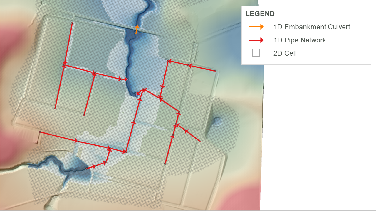
Figure 3.1: 1D Pipe Network and Embankment Culvert Linked to 2D

• 1D is used for open channel modelling where the 2D resolution is too coarse to represent the open channel shape. The 1D open channels are linked to a 2D domain covering the surface inundation of adjacent floodplain areas. An example of this configuration is shown in Figure 3.2. Refer to TUFLOW Tutorial Module 11 for a model demonstration.

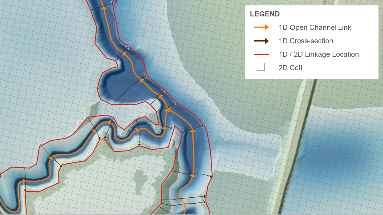
Figure 3.2: 1D Open Channel Linked to 2D

Despite the above, the advent of faster computers, GPU acceleration and Sub-Grid Sampling (SGS) has seen open channels increasingly represented in the 2D domain in TUFLOW models. The key drivers for this are:

• Computing power increases, combined with TUFLOW HPC’s GPU acceleration, have enabled models built today to be over 100 times larger than pre 2018 models (in terms of cell count). The increased computing power means modellers can model at a finer resolution and over larger areas with no simulation time penalties.
  
• The development of HPC’s 2D Sub-Grid Sampling (see Section 3.2.3), which creates more accurate storage curves for cells and flux area curves for faces, has vastly improved the ability of a 2D model to reasonably predict the hydraulic conveyance of surface channels. SGS is built into all of the TUFLOW Tutorial Modules.
• The development of HPC’s 2D quadtree grid refinement permits use of finer resolution 2D cells in discrete regions (see Section 3.1.4), such as within the open channel areas.

Section 10 provides a detailed description of how to implement 1D-2D linking and exploit the above within the TUFLOW suite of products.

3.1.4 Quadtree Grid

By default TUFLOW Classic and HPC use a single 2D cell resolution over an entire model domain. This type of configuration is referred to as a fixed grid configuration. To support 2D modelling at a range of spatial resolutions (which is often a project requirement), TUFLOW HPC models can use a quadtree grid or mesh. The quadtree grid refinement feature supports the recursive division of square TUFLOW cells into four smaller square cells. Up to nine levels of cell size refinement are permitted. All cells in all levels of refinement share a common orientation and the hydraulic computations are a full 2D solution across the entire quadtree grid.

An example quadtree grid is presented in Figure 3.3 and detailed documentation is provided in Sections 7.3.1 and 10.7.1. TUFLOW Tutorial Module 7 provides a demonstration of this model configuration feature.

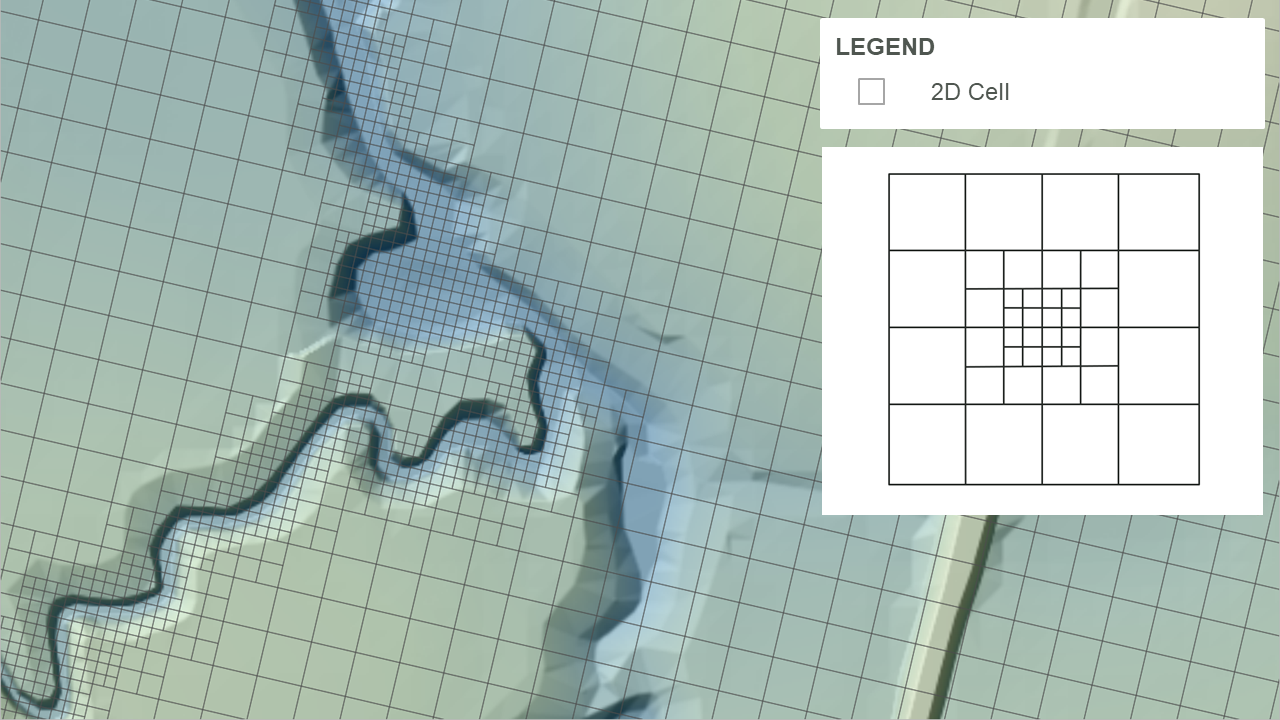
Figure 3.3: TUFLOW HPC Quadtree Grid (3 Level Refinement)