3.3 Solution Accuracy

Solving the shallow water equations in one or two dimensions is necessarily an approximation and there are numerous solutions and different assumptions to be made. The following sections discuss various forms of the shallow water equations. Of these, TUFLOW adopts the full dynamic wave form in its 1D and 2D solutions. The full dynamic wave solution is the most accurate option compared to the other mentioned alternative solution schemes.

3.3.1 Fluid Flow Physical Terms

The equations solved by TUFLOW are:

• Conservation of mass (also known as the continuity equation)
• Conservation of momentum

These equations are presented and discussed in 1D and 2D forms in the subsections below.

3.3.1.1 1D Continuity Equation

For water flow within a 1D channel the continuity equation per unit length is:

\[\begin{equation} \begin{matrix} w \frac{\partial h}{\partial t} & + & \frac{\partial (A u)}{\partial x} & = & S(x) \\ \text{rate} & + & \text{divergence} & = & \text{source} \end{matrix} \tag{3.1} \end{equation}\]

Where

• \(w\) is the channel width at the water surface
• \(h\) is the water depth in the channel
• \(A\) is the cross-sectional flow area (up to the water surface)
• \(u\) is the cross-sectional flow area averaged water velocity
• \(S(x)\) is the lineal water source term (volume per unit time per unit length), usually lateral inflow/outflow
• \(x\) and \(t\) are channel flow dimension and time respectively

3.3.1.2 1D Momentum Equation

For water flow within a 1D channel the momentum equation is as follows, noting the eddy viscosity (diffusion of momentum or turbulence) term can not be included in the 1D form.

\[\begin{equation} \begin{matrix} \frac{\partial u}{\partial t} & + & \frac{1}{A} \frac{\partial (Auu)}{\partial x} & + & g \frac{\partial (z+h)}{\partial x} & + & g \frac{n^2|u|}{R^\frac{4}{3}}u & = & S_u(x) \\ \text{rate} & + & \text{divergence} & + & \text{slope} & + & \text{friction} & = & \text{source} \end{matrix} \tag{3.2} \end{equation}\]

Where

• \(z\) is the channel bed elevation
• \(n\) is the Manning’s coefficient for bed friction (units time per cube-root(unit length))
• \(R\) is the hydraulic radius
• \(g\) is acceleration due to gravity
• \(S_u(x)\) is the lineal momentum source term (force per unit volume per unit fluid density), typically used for local energy losses unable to be represented by the 1D form

Note the hydraulic radius \(R\) is normally considered to be cross-sectional flow area divided by wetted perimeter, or \(A/P\). However, in some software it may be specified as ‘resistance radius’, which is just the water depth over the channel invert.

3.3.1.3 2D Continuity Equation

For water flow over a 2D surface the continuity equation is:

\[\begin{equation} \begin{matrix} \frac{\partial h}{\partial t} & + & \frac{\partial (h u)}{\partial x} & + & \frac{\partial (h v)}{\partial y} & = & S(x,y) \\ \text{rate} & + & \text{divergence} & + & \text{divergence} & = & \text{source} \end{matrix} \tag{3.3} \end{equation}\]

Where

• \(h\) is the water depth in the 2D cell
• \(u\) and \(v\) are the velocity components in the \(x\) and \(y\) spatial dimensions, respectively
• \(S(x,y)\) is the total area water source term (volume per unit time per unit area), usually rain and infiltration

3.3.1.4 2D Momentum Equation

For water flow over a 2D surface the momentum equations, including eddy viscosity (diffusion of momentum or turbulence) but omitting Coriolis acceleration \(\Omega\), are:

\[\begin{equation} \begin{matrix} \frac{\partial (hu)}{\partial t} & + & \frac{\partial (huu)}{\partial x} + \frac{\partial (hvu)}{\partial y} & - & \frac{\partial (h \nu_t \frac{\partial u}{\partial x})}{\partial x} - \frac{\partial (h \nu_t \frac{\partial u}{\partial y})}{\partial y} & + & gh \frac{\partial (z+h)}{\partial x} & + & gh \frac{n^2\sqrt{u^2+v^2}}{h^\frac{4}{3}}u & = & S_u(x,y) \\ \frac{\partial (hv)}{\partial t} & + & \frac{\partial (huv)}{\partial x} + \frac{\partial (hvv)}{\partial y} & - & \frac{\partial (h \nu_t \frac{\partial v}{\partial x})}{\partial x} - \frac{\partial (h \nu_t \frac{\partial v}{\partial y})}{\partial y} & + & gh \frac{\partial (z+h)}{\partial y} & + & gh \frac{n^2\sqrt{u^2+v^2}}{h^\frac{4}{3}}v & = & S_v(x,y) \\ \text{rate} & + & \text{divergence} & - & \text{diffusion} & + & \text{slope} & + & \text{friction} & = & \text{source} \end{matrix} \tag{3.4} \end{equation}\]

Where

• \(\nu_t\) is the (kinematic) turbulent eddy viscosity
• \(S_u(x,y)\) and \(S_v(x,y)\) are the areal momentum source terms (force per unit area per unit fluid density), used for local energy losses and atmospheric pressure gradient

3.3.2 Forms of the Equations

Equations (3.1) and (3.2) are the 1D Dynamic Wave Equations, or Saint-Venant Equations. They represent a system of equations that is effectively second order in both space and time, and admit travelling wave solutions (speed \(c=\sqrt{gh}\)). Similarly Equations (3.3) and (3.4) are the 2D Dynamic Wave Equations also known as the Shallow Water Equations (SWE).

As described in the following subsections, the Dynamic form of the equations can be simplified to the Diffusive and Kinematic forms. However, given the available computing power today in personal computers, there is no need or defence for calculating diffusive wave or kinematic wave solutions except for very specific simplified situations. TUFLOW Classic and HPC are strictly dynamic wave solvers, in both 1D and 2D forms. TUFLOW does not experience the inaccuracies and limitations associated with solving the diffusive wave or kinematic wave equations.

3.3.2.1 Diffusive Wave Equation

In the case of 1D, the two prognostic variables, depth \(h\) and velocity \(u\) co-evolve with time. However, in days past when computers were far less powerful, the Dynamic Wave Equation solution was computationally too much work to solve efficiently. At that time in history mathematicians looked to simplify the problem. The first step was to assume that the velocity field is a “slowing evolving steady state solution” (i.e. the time derivative \(\frac{\partial u}{\partial t}\) is considered small and the velocity field is no longer independently evolved); it becomes a diagnostic field that is able to be computed from the depth field. Further, by assuming that solution is “gentle” (i.e. the divergence term \(\frac{1}{A} \frac{\partial (Auu)}{\partial x}\) is also small), the velocity field can be defined as:

\[\begin{equation} |u|u = -\frac{R^\frac{4}{3}}{n^2} \frac{\partial (z + h)}{\partial x} \tag{3.5} \end{equation}\]

Equation (3.1), with the velocity field computed diagnostically from (3.5) is the 1D Diffusive Wave Equation. The equation is second order in space but only first order in time. It does not admit travelling wave solutions, but solutions that diffuse while they advect, hence the name. It requires less memory, less computational effort per timestep, and a larger timestep can be used to progress forward in time compared to the dynamic wave solution.

In situations where the velocity field is gentle and slowly evolving, the Diffusive Wave solution is almost correct. However, as the modeller cannot know in advance just how large the difference between the diffusive and dynamic wave solutions might be, sensitivity testing by comparing results using the two forms is recommended, or the Diffusive form is simply not used.

Diffusive wave solutions are also not shock capturing, and do not accurately predict the location of hydraulic jumps. In 2D the diffusive wave solution is even more incorrect. As the divergence of momentum in both \(x\) and \(y\) is neglected, the solution cannot estimate super-elevation.

For the reasons above, TUFLOW’s solvers do not offer a Diffusive Wave solution.

3.3.2.2 Kinematic Wave Equation

From the diffusive wave equation solution, there are further simplifications that are possible and sometimes used by other software. For shallow flows over steeper ground it is possible to assume that \(\partial h / \partial x\) << \(\partial z / \partial x\), in which case the velocity field becomes a function of depth and channel bed slope, but not a function of \(\partial h / \partial x\). The equation then becomes first order in both space and time:

\[\begin{equation} w \frac{\partial h}{\partial t} + \frac{\partial (A B R^\frac{2}{3})}{\partial x} = S(x) \\ B = \frac{1}{n} {\left| \frac{\partial z}{\partial x} \right|}^\frac{1}{2} sgn \left( \frac{\partial z}{\partial x} \right) \tag{3.6} \end{equation}\]

Equation (3.6) is the 1D Kinematic Wave Equation. It is a non-linear advection equation. It is suitable for computing steady state flows (and slowly evolving steady state flows) in steep channels or over steep terrain (i.e. water surface slope is much the same as bed slope), but is not suitable for flows in low-lying channels/rivers.

For the reasons above, TUFLOW’s solvers also do not offer a Kinematic Wave solution.

3.3.3 Numerical Accuracy

When computing the divergence and diffusion terms in a finite difference or finite volume scheme, it is necessary to calculate the field values at spatial locations that are between the locations where the field data are defined. For example, depth data is considered a node or cell property, and is nominally defined at a node (1D) or cell centre (2D). When calculating the flow through a cross-section (1D) or a face (2D), the depth of water must be estimated at the cross-section (or face), which is located between the nodes (or cells). This process is not straight forward, the methods for doing so broadly fall into three categories:

• Zeroth order interpolation: The field value used at the cross-section or a face is a constant fixed value. This means that the error between the field value used and the “real” solution is constant regardless of cell size - it is a function of cell size to the power of zero, hence the term “zeroth order”. This method is generally not used.
  

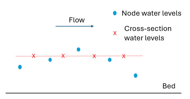
  Figure 3.10: Example of zeroth order interpolation

• First order interpolation: The field value used at the cross-section or a face is usually that of the upwind (upstream) node or cell, but in rare cases can be that of the downwind (downstream) node/cell. This means that the error between the field value used and the real solution is proportional to the 1D element length or 2D cell size it is a function of element length or cell size to the power of one, hence the term “first order”. This method is computationally simple and is very stable, but has the tendency to cause any sudden changes (high spatial gradients) in solution to diffuse (smooth out) over time - the same effect as if the model had a high diffusion rate applied. The method introduces an artefact diffusion that isn’t real. In the case of 2D and 3D modelling, any swirls or eddies in the velocity field tend to decay (or simply do not form in the first place).

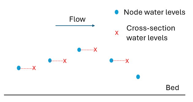
Figure 3.11: Example of first order interpolation

• Second order interpolation: The field value used at the cross-section or a face is usually linearly interpolated between the upwind node/cell and the downwind one. This means that the error between the field value used and the real solution is proportional to element length or cell size squared - it is a function of cell size to the power of two, hence the term “second order”. Pure linear interpolation on its own is known to be unstable - the solution tends to develop oscillations in locations with high gradients. To prevent these, it is common to blend between first and second order interpolation depending on the spatial gradients relative to the grid/mesh size - this is known as rate limiting, or a Total Variation Diminishing (TVD) method. When implemented correctly, the level of artefact numerical diffusion is very small, and swirls and eddies in the velocity field (2D and 3D) form easily unless real diffusion (such as a turbulence model) is explicitly added.
  

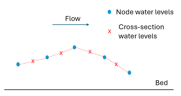
  Figure 3.12: Example of second order interpolation

TUFLOW Classic uses second order interpolation, and TUFLOW HPC defaults to second order interpolation, but does offer the user the choice to switch to first order (see Solution Scheme). However, for the reasons above using a first order interpolation solution is not recommend. Second order interpolation is significantly more accurate than first order, and this shows in cell-size sensitivity testing. The TVD scheme implemented in TUFLOW HPC is very stable, and the user should not need to change to first order interpolation in order to stabilise a model.