3.4 Timestep
Appropriate computational timestep selection is critically important for the successful stable simulation of a model. In hydraulic modelling the timestep represents the interval at which the hydraulic calculations proceed forward in time. From a model design perspective it influences both the simulation stability and overall runtime considerations.
Depending on the numerical construct and solution scheme there are critical control number criterion that must not be exceeded to maintain solution stability. Additionally, the simulation run time is directly proportional to the number of timesteps required to calculate model behaviour for the simulation period. Selecting a timestep that is too large, exceeding the relevant control number criterion, may cause computations to become unstable. Conversely, selecting a timestep that is excessively small will unnecessarily slow a simulation down. The following sections provides timestep selection guidance.
3.4.1 Fixed versus Adaptive Timestepping
There are typically two approaches to how a model’s timestep is applied:
- Fixed Timestepping: The timestep is determined and input as a fixed value by the user. For TUFLOW modelling, this approach applies to TUFLOW Classic.
- Adaptive Timestepping: The timestep is automatically determined by the solution scheme and varies in value throughout the simulation depending on the hydraulic conditions at the time. TUFLOW HPC uses adaptive timestepping.
Note: TUFLOW’s in-built 1D solutions, TUFLOW 1D (ESTRY) and EPA SWMM, use a variety of fixed and adaptive timestepping, depending on the 2D solution it is linked to (TUFLOW Classic or HPC).
3.4.2 TUFLOW 1D (ESTRY) and EPA SWMM
TUFLOW 1D (ESTRY) and EPA SWMM both use an explicit solution scheme. For the 1D channels using either of these solvers the stability criterion, expressed by the following wave celerity (3.7) and courant number (3.8) equations, should not exceed 1.
\[\begin{equation} C_c = \frac{\Delta t \sqrt{gh}}{\Delta x} \tag{3.7} \end{equation}\]
\[\begin{equation} C_u = \frac{\Delta t \cdot U }{\Delta x} \tag{3.8} \end{equation}\]
Where:
- \(Cc\) = Wave celerity
- \(Cu\) = Courant number
- \(\Delta t\) = Timestep
- \(\Delta x\) = Distance
- \(g\) = Gravity
- \(h\) = Water depth
- \(U\) = Magnitude of velocity
The ESTRY Control File Timestep command is used to set the fixed TUFLOW 1D (ESTRY) timestep, or when linked with HPC, the maximum 1D timestep.
The TUFLOW SWMM Control File SWMM Iterations command sets the EPA SWMM timestep relative to the linked 2D solution timestep.
A fixed TUFLOW 1D (ESTRY) timestep is recommended for 1D/2D linked TUFLOW Classic models. The timestep selected should not be greater than the minimum value for any channel (except non-inertial channels such as bridges, culverts, etc.). Typical timestep values are 10 or 60 seconds for a model with a minimum channel length of 100 to 500 metres, down to 1 second for 1D network with small pipes. The occurrence of mass errors may indicate the use of too high a timestep.
Tip: Where a few TUFLOW 1D (ESTRY) channels must be significantly shorter than the rest, it may be economical to specify them as non-inertial channels. The timestep can then be chosen on the requirements of the shortest remaining channel. Care should however be exercised when specifying non-inertial channels to ensure that errors are not introduced by the non-inertial representation, particularly if these channels are in a region of interest. Any approximations can usually be assessed by a few selected runs without the non-inertial approximation and with the necessary shorter timestep.
In 1D/2D linked TUFLOW Classic models a TUFLOW 1D (ESTRY) Timestep value that is smaller and also equally divisible into the 2D Timestep is recommended. If the 1D timestep is not equally divisible into the smallest 2D timestep, the 1D timestep is reduced automatically so that it meets this criteria. For example, if the specified 2D timestep is 10 seconds and the 1D timestep is 3 seconds, the 1D timestep will be reduced to 2.5 seconds (this is reported in the simulation log file).
A fixed timestep is also required as the model input for 1D/2D linked TUFLOW HPC models, though functionally during simulation, timestep adjustment is applied to enable synchronised communication between TUFLOW 1D (ESTRY) and TUFLOW HPC’s adaptive timestep. In this situation the TUFLOW 1D (ESTRY) Timestep represents a “Maximum 1D Timestep”. The timestep synchronisation is shown Figure 3.13, and functions as follows:
- If the TUFLOW HPC 2D Timestep is greater than the Maximum TUFLOW 1D (ESTRY) Timestep: the 1D timestep is reduced to an integer division of the 2D timestep. For example, if the HPC 2D timestep is 1.2 s, and the ESTRY/SWMM 1D maximum timestep is 1.0 s, then ESTRY will use 0.6 s for its timestep and run two steps to HPC’s single step.
- If the TUFLOW HPC 2D Timestep is less than the Maximum TUFLOW 1D (ESTRY) Timestep: the 1D timestep is reduced to synchronise with the 2D timestep. The two cases are as follows:
- If the 2D timestep is greater than half the 1D timestep but less then the 1D timestep (i.e. 0.5 * Maximum TUFLOW 1D Timestep < TUFLOW HPC 2D Timestep < Maximum TUFLOW 1D Timestep), then the reduced 1D timestep is synchronised with every 2D timestep.
- If the 2D timestep is less than half the 1D timestep (i.e. TUFLOW HPC 2D Timestep < 0.5 * Maximum TUFLOW 1D Timestep), then the 1D timestep is synchronised with a multiple of the 2D timestep.
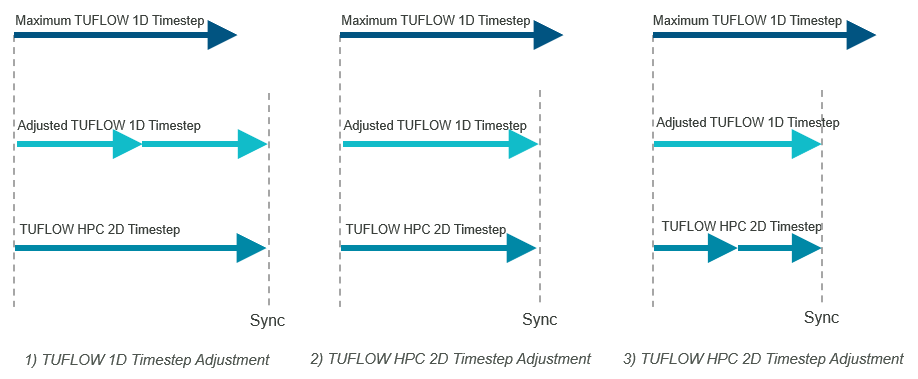
Figure 3.13: TUFLOW HPC 1D/2D Timestep Synchronisation
3.4.3 TUFLOW Classic 2D
TUFLOW Classic is a 2D implicit scheme. It can generally maintain a stable solution for a Courant Number (Equation (3.9)) less than 10. For real-world applications a value of 5 or less is however more common (Syme, 1991).
\[\begin{equation} \text{C}_{\text{r}} = \frac{\Delta t\sqrt{2\text{gH}}}{\Delta x} \tag{3.9} \end{equation}\]
Where:
- \(\Delta t\) = Timestep (s)
- \(\Delta x\) = Length of model element (m or ft)
- \(g\) = Acceleration due to gravity (\({ms}^{- \frac{1}{2}}\))
- \(H\) = Depth of water (m or ft)
Note: Metric (SI) units are TUFLOW’s default. To use imperial units, ensure
As a general rule for 2D TUFLOW Classic models, the Timestep (in seconds) is typically in the range of \(\frac{1}{2}\) to \(\frac{1}{5}\) of the cell size (in metres). For example, for a 10m model the timestep will typical be in the range 2 to 5 seconds. For steep gradient models with high Froude numbers and supercritical flow, smaller timesteps may be required.
If a model is operating at high Courant numbers (>10), sensitivity testing with smaller timesteps to demonstrate no measurable change in result is recommended. The occurrence of high 2D mass error can be an indicator that the 2D timestep is too high.
Tip: If during initial model development a model becomes unstable, it is strongly advised to not simply reduce the timestep. Instead establish why the model is unstable and if the cause relates to poor model design or one of the model input error (e.g topography, boundary conditions, initial water level, 1D/2D linking etc.). If it is, correct that first before considering lowering the timestep. Doing so will create a healthy model that can operate at a higher timestep, and subsequently run faster. Section 16.3 includes guidance focused on resolving model instabilities.
3.4.4 TUFLOW HPC 2D
TUFLOW HPC is a 2D explicit scheme. It uses adaptive timestepping to progress through a simulation. The timestep is automatically dynamically adjusted during a simulation so the numerical solution complies with three mathematical stability criteria, shown in Table 3.2.
| Control Number | Description | Expression and Control Limit Maximum |
|---|---|---|
| Courant Number (Nu) | This condition ensures that water entering one side of a 2D cell does not pass through the other side within one timestep. For this to be satisfied, the product of the water velocity (\(\upsilon\), \(\nu\)) and model timestep (\(\Delta\)t) must be less than the cell size (\(\Delta\)\(x\), \(\Delta\)\(y\)) . | \[\begin{equation} max(\frac{|\upsilon|\Delta t}{\Delta x} , \frac{|\nu|\Delta t}{\Delta y}) = 1.0 \end{equation}\] |
| Shallow Wave Celerity Number (Nc) | This numerical condition relates to the shallow water wave celerity (wave speed) and is derived from the fluid flow equations to represent long waves (i.e. wave length is substantially longer than the water depth). The product of the model timestep (\(\Delta\)t) and the long wave speed (square root of the gravity (\(g\)) and water depth(\(h\))) must be less than the cell size (\(\Delta\)\(x\), \(\Delta\)\(y\)), for the condition to be satisfied. | \[\begin{equation} max(\frac{\sqrt{2\text{gh}}\Delta t}{\Delta x} , \frac{\sqrt{2\text{gh}}\Delta t}{\Delta y}) = 1.0 \end{equation}\] |
| Diffusion Number (Nd) | This numerical condition relates to the sub-grid scale eddy viscosity term which causes diffusion of momentum. To maintain stability the product of the eddy viscosity coefficient (\(\text{v}_{\tau}\)) and the timestep (\(\Delta\)t) divided by the square of the grid spacing (\(\Delta\)\(x\), \(\Delta\)\(y\)) must remain below 0.3. | \[\begin{equation} max(\frac{\text{v}_{\tau}\Delta t}{\Delta x^2} , \frac{\text{v}_{\tau}\Delta t}{\Delta y^2}) = 0.3 \end{equation}\] |
TUFLOW HPC will use the highest timestep possible without exceeding the limits associated with each of the above control numbers. The method TUFLOW HPC uses to calculate a timestep and achieve unconditional stability is as follows:
- A TUFLOW Control File (TCF) Timestep command is required. It is however only used for the first calculation timestep. The specified value should be consistent with what would be appropriate for a TUFLOW Classic model (i.e. \(\frac{1}{2}\) to \(\frac{1}{5}\) the 2D cell size in metric units). Internally, TUFLOW HPC divides this value by 10 to apply a value that is suitable for an explicit solution scheme. All subsequent calculations are completed using the adaptive timestep approach outlined in the following bullet points.
- The HPC timestep is calculated using the hydraulic conditions from the end of the previous timestep.
- If the hydraulic conditions have changed significantly it is possible for one or more of the Nu, Nc, Nd control number criteria to be violated at one or more locations within the model. For example, a sudden change in rainfall from one timestep to the next (which occurs with stepped rainfall boundaries) would potentially cause this. The HPC solver, by default, treats a 20% exceedance of a control number as a violation and will implement a repeat timestep feature in this situation in order to maintain unconditional stability. Should a control number anywhere within the model be exceeded by more than 20%, the solution reverts to the complete hydraulic solution from the previous (good) timestep, then the timestep is reduced and next calculation repeated.
- Each timestep is also tested for the occurrence of NaNs. A NaN is “Not a Number” and occurs due to undefined mathematical calculations such as a divide by zero or square root of a negative number. The occurrence of a NaN is also indicative of a sudden instability. Should a NaN occur, the repeat timestep feature is implemented.
- Should a timestep need to be repeated more than ten times consecutively, the solution stops.
- The simulation will also stop if the default minimum permissible timestep of 0.1 seconds has been reached. This value can be manually adjusted using Timestep Minimum.Repeated timesteps are displayed to the Console Window and the number of them for a time interval are provided in the nRS_NaNs and nRS_HCNs columns in the _HPC.csv file output in the results folder. They are also reported to the _messages layer.
Internally, HPC multiplies the Nu, Nc, Nd control number limits by a dynamic control factor. This factor starts at 1.0 at the beginning of a simulation, and normally will stay at 1.0, unless a repeat timestep occurs. If a repeat timestep occurs, this factor is reduced to 90% of its previous value, thereby decreasing all of the control number limits. The dynamic factor very slowly increases again with each good timestep, up to a maximum value of 1.0. HPC offers two methods, via the HPC Timestep Approach command, for the calculation of whether a “high control number” event has occurred. ‘Method A’ considers that a high control number step has occurred if any of Nu, Nc, Nd has exceeded the dynamic control number limits (i.e. after the dynamic control factor has been applied) by the 20% margin. Whereas ‘Method B’ (introduced in the 2025 release and set as the new default) applies the test using the original static limits (i.e. before the dynamic control factor has been applied). Method B is more tolerant in models that have rapid wetting and drying.
Repeated timesteps may be an indication the solution is numerically “on-the-edge”. Models that have a high number of repeated timesteps should be sensitivity tested by reducing the control number limits using Control Number Factor. For example, repeat the simulation using
Tip: Reviewing the TUFLOW HPC minimum timestep output is a useful way to assess HPC model health. Models that reduce to an excessively small 2D timestep in order to remain stable may be symptomatic of an unhealthy model. Identifying what the limiting control number is that is causing the timestep requirement can provide clues to the model feature to review for errors. For example:
- Celerity Control (Nc) number relates to water depth relative to cell size. Energy can pass through deeper water faster than shallow water, as such deep water will trigger this control. Review whether the water depth is realistic, or the result of an error in the model topography.
- Courant number (Nu) relates to velocity relative to the cell size. High velocities will trigger this as the control. Investigate whether the feature causing the high velocity is realistic.
- Diffusion control (Nd) relates diffusion of momentum relating to the sub grid viscosity. Small cells in deep water will trigger this one. Models controlled by the diffusion number tend to require a timestep significantly smaller than those controlled by the shallow wave celerity or courant numbers. If a model is predominantly diffusion controlled it may be that equivalent solution accuracy can be achieved by selecting a larger cell size. This is worth testing, as it will most likely increase the simulation speed with no loss of result fidelity.
Section 16.3 includes guidance focused on reviewing model health and resolving issues.
3.4.4.1 Timestep Efficiency Output
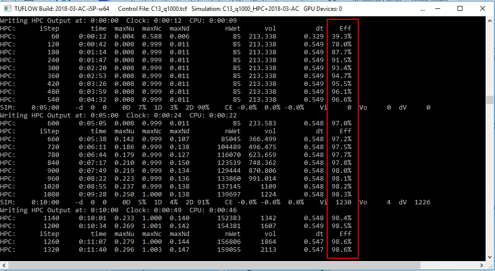
A timestep efficiency result is output for HPC simulations, reported to the console window, HPC log file (.hpc.tlf) and the timestep history file (.dt.csv). A value of 100% indicates that the HPC timesteps are perfectly aligned with the minimum stability timestep for complying with the three control numbers listed in Table 3.2. Factors that reduce the timestepping efficiency can be:
- Lower initial timestep than required. This will be evident by low values at the start, then steadily increasing towards 100% as the timestep approaches the optimum value – see example further below.
- Synchronisation with a 1D scheme. The 1D/2D linking with TUFLOW’s 1D solver (ESTRY) is designed to synchronise exactly using the larger of the 1D or 2D timesteps. For external 1D schemes, the timestepping is similarly synchronised, with some external 1D schemes also offering an unsynchronised option. In all cases, the HPC 2D timestepping will be below optimum by varying degrees, with the inefficiency shown in the timestepping efficiency output.
- Frequent map or time-series output. The HPC timestepping is configured to align exactly with map and time-series output intervals. Timesteps nearly always need to be reduced as an output interval is approached. These reduced timesteps can be found in the “dt” column of the hpc.dt.csv file. The ideal timestep without the output interval reductions is reported in the “dtStar” column.
For example, in the output window below, the efficiency is initially poor (~40%) due to the initial timestep in the model being too low, however the efficiency rapidly increases as the HPC timestep increases.
Note: Should a model exhibit low overall timestepping efficiency (i.e. values less than around 70 to 90%), please let us know via support@tuflow.com, and attach the .tlf, .hpc.tlf and dt.csv files.