9.2 1D Domains
9.2.1 1D Cross-Sectional Averaged Equation of Motion
The movement of constituents through 1D (ESTRY) channels is supported via SX connections. Prior to the 2025 release, movement of constituents through these connections was only on a mass balance basis. That is, it assumed that the concentration of a constituent exiting an SX connection is the same as that at the entrance SX connection, at the same timestep. While this provides a simplified method to pass constituents through relatively ‘short’ 1D channels, it does not consider the time taken for the constituents to flow over the distance of a 1D channel, nor the mixing of water with different tracer concentrations at 1D channel junctions.
The 2025 release introduced a new approach to partially support the advection of constituents in 1D channel networks. The mass balance equation is solved by taking into account the velocity in 1D channels and the water volume at 1D nodes. The travel time of the constituents through 1D channel and the mixing of constituents at 1D junctions are now simulated properly. This new approach is set as default in the 2025 release by the following ecf command:
Backward compatibility is offered by setting this command to ‘Method A’.
When Method B (the default) is used, the equation of motion of a passive tracer \(\phi\) (as a concentration) in 1D ESTRY channels is solved as:
\[\begin{equation} \frac{\partial(A \phi)}{\partial t} + \frac{\partial(A u \phi)}{\partial x} - \frac{\partial}{\partial x} \left( A D_x \frac{\partial \phi}{\partial x} \right) = A S_\phi \tag{9.15} \end{equation}\]
Where:
- \(\phi\) = Tracer concentration as mass (or mols) per unit volume
- \(A\) = Cross-sectional flow area (up to the water surface)
- \(u\) = Cross-sectional averaged velocity components in the x direction
- \(x\) = 1D spatial coordinates in the streamwise direction
- \(t\) = Time
- \(D_x\) = Isotropic dispersion plus turbulent diffusion coefficients values in the x direction
- \(S_\phi\) = Tracer source as mass (or mols) per unit volume per unit time
9.2.2 1D Solution Method (ESTRY)
The TUFLOW 1D (ESTRY) AD solver is based on the implicit finite volume method. Equation (9.15) is integrated over the 1D nodal volume, from the channel mid-section of the upstream channel to the mid-section of the downstream channel, i.e. the same 1D node ESTRY uses to store water volume. The tracer concentration at node \(i\), at the next timestep is calculated as:
\[\begin{equation} \phi_{i,n+1} = \phi_{i,n} + \Delta t \frac{\sum{Q \phi}}{V_{i}} \tag{9.16} \end{equation}\]
Where:
- \(\phi_{i,n+1}\) = Tracer concentration at node \(i\) at next timestep
- \(\phi_{i,n}\) = Tracer concentration at node \(i\) at current timestep
- \(\Delta t\) = Timestep
- \(Q\) = Cross-sectional volumetric flux at the connected channel mid-sections
- \(\phi\) = Tracer concentration the connected channel mid-sections
- \(V_{i}\) = 1D nodal water volume at node \(i\) (up to the water surface)
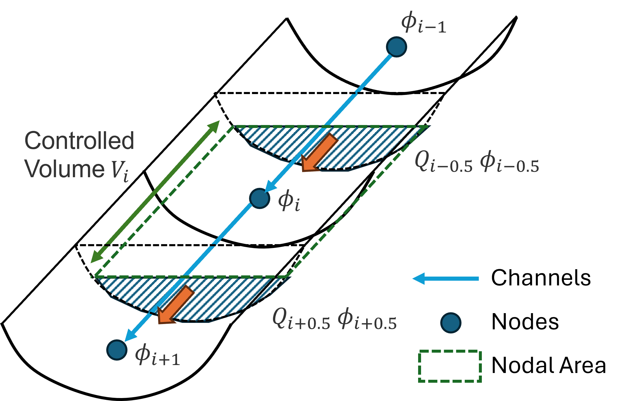
Figure 9.1: 1D Channel Advection
ESTRY solves flux/velocity at channel mid-section, so spatial interpolation is not needed for \(Q\). The mid-section concentration \(\phi\), on the other hand, is interpolated from the nodal concentration using 2nd order spatial scheme with Superbee gradient limiter (Fringer et al., 2005).