5.7 Structures
Hydraulic structures in the 1D domain are modelled by replacing the momentum equation with standard equations describing the flow through the structure. The structures available are described in the following sections. A discussion on the choice of a 1D or 2D representation of the structure is presented in Section 7.2.10.1.
A channel is flagged as a hydraulic structure using the Type attribute as described in Table 5.1. Except for culverts, a structure has zero length, i.e. there is no bed resistance. If a non-zero length is applied to a “zero length” structure, this is only used in the calculation of the storage (nodal area).
5.7.1 Culverts and Pipes
Culvert or pipe channels can be either rectangular, circular (pipe) or irregular in shape. A range of different flow regimes is simulated with flow in either direction. Adverse slopes are accounted for and flow may be subcritical or supercritical. Figure 5.4, Figure 5.5 and Table 5.6 present the different flow regimes which can be modelled. The regimes that occur during a simulation are output to the .eof file next to the velocity and flow output values, and to the _TSF GIS layer (see Sections 14.5 and 15.2.4), and can be displayed on time-series plots in the QGIS TUFLOW Viewer plugin.
For all culvert types the length, upstream and downstream inverts, Manning’s n, bend loss, entrance and exit losses, and number of barrels are entered using the 1d_nwk attributes (see Table 5.5). For type “C” circular or type “R” rectangular culverts, the dimensions are also specified within the 1d_nwk attributes. For an “I” irregular shaped culvert, the cross-sectional shape is specified using a 1d_xs GIS layer and the Read GIS Table Links command. The line must be digitised across the 1d_nwk channel line using the mid cross-section approach (refer to Section 5.6.5 and Table 5.4). This is the only supported approach for structures such as irregular shaped culverts, bridges, and weirs.
The four culvert coefficients are as follows:
- The height contraction coefficient for box culverts. Usually 0.6 for square edged entrances to 0.8 for rounded edges. This factor is not used for circular culverts.
- The width contraction coefficient for box culverts. Typically values from 0.9 for sharp edges to 1.0 for rounded edges. This factor is normally set to 1.0 for circular culverts.
- The entry loss coefficient. The standard value for this coefficient is 0.5. Variations to this value may be applied based on manufacturer specifications.
- The exit loss coefficient, normally recommended as 1.0.
The calculations of culvert flow and losses are carried out using techniques from “Hydraulic Charts for the Selection of Highway Culverts” and “Capacity Charts for the Hydraulic Design of Highway Culverts”, together with additional information provided in Henderson (1966). The calculations have been compared and shown to be consistent with manufacturer’s data provided by both “Rocla” and “Armco”.
Note: By default, the entrance and exit losses above are adjusted every timestep according to the approach and departure velocities based on the equations in Section 5.7.7.
For benchmarking of culvert flow to the literature, see “TUFLOW Validation and Testing” (Huxley, 2004).
| No. | Default GIS Attribute Name | Description | Type |
|---|---|---|---|
| 1 | ID |
Unique identifier up to 12 characters in length. It may contain any character except for quotes and commas, and cannot be blank. As a general rule, spaces and special characters (e.g. “\”) should be avoided, although they are accepted. The same ID can be used for a channel and a node, but no two nodes and no two channels can have the same ID. When automatically creating nodes (default) “.1” and “.2” are added to the channel names for the upstream and downstream node names respectively. IDs over 10 characters long are not recommended as the appending of .1 and .2 can cause duplicate node ID’s to be created. |
Char(12) |
| 2 | Type |
The culvert type:
|
Char(4) |
| 3 | Ignore | If a “T”, “t”, “Y” or “y” is specified, the object will be ignored (T for True and Y for Yes). Any other entry, including a blank field, will treat the object as active. | Char(1) |
| 4 |
UCS (Use Channel Storage at nodes) |
If left blank or set to Yes (“Y” or “y”) or True (“T” or “t”), the storage based on the width of the channel over half the channel length is assigned to both of the two nodes connected to the channel. If set to No (“N” or “n”) or False (“F” or “f”), the channel width does not contribute to the node’s storage. See Section 5.12 for further discussion. | Char(1) |
| 5 | Len_or_ANA | The length of the culvert in metres. If the length is less than zero, except for the special values below, the length of the line is used. | Float |
| 6 | n_nF_Cd |
The Manning’s n value of the culvert. If using materials to define the bed resistance from XZ tables (only for Irregular culvert, see Section 5.6.1.1.2), n_nF_Cd should be set to one (1) as it becomes a multiplication factor of the materials’ Manning’s n values. It may be adjusted as part of the calibration process. |
Float |
| 7 | US_Invert |
The upstream bed or invert elevation of the culvert in metres. If a culvert invert has a value of -99999 (after any application of node/pit DS_Invert values), the invert is interpolated by searching upstream and downstream for the nearest specified inverts, and the invert is linearly interpolated. Interpolate Culvert Inverts can also be used to switch this feature ON or OFF. |
Float |
| 8 | DS_Invert | Sets the downstream invert of the culvert using the same rules as for described for the US_Invert attribute above. | Float |
| 9 | Form_Loss |
Specifies an additional dynamic head loss coefficient that is applied when the culvert flow is not critical at the inlet. This applies the energy loss appropriately for a ‘minor’ loss using K*V2/2g. Bend loss coefficients (K) are found in many standard hydraulic references. Note, this loss coefficient is not subject to adjustment when using |
Float |
| 10 | pBlockage |
C, R Channel Type: I Channel Type: |
Float |
| 11 | Inlet_Type | Not used. | Char(256) |
| 12 | Conn_1D_2D | Not used. | Char(4) |
| 13 | Conn_No | Not used. | Integer |
| 14 | Width_or_Dia |
C Channel Type: R Channel Type: Not used. |
Float |
| 15 | Height_or_WF |
R Channel Type: Not used. |
Float |
| 16 | Number_of | The number of culvert barrels. If set to zero, one barrel is assumed. | Integer |
| 17 | HConF_or_WC |
I, R Channel Type: Not used. |
Float |
| 18 | WConF_or_WEx |
The width contraction coefficient for inlet-controlled flow. Usually 0.9 for sharp edges to 1.0 for rounded edges for R culverts. Normally set to 1.0 for C culverts. If value exceeds 1.0 or is less than or equal to zero, it is set to 1.0 for C and 0.9 for R culverts. Not used for outlet controlled flow regimes. |
Float |
| 19 | EntryC_or_WSa |
The entry loss coefficient for outlet controlled flow (recommended value of 0.5). If value exceeds 1.0, it is set to 1.0. If value is less than zero (0), it is set to zero (0). If |
Float |
| 20 | ExitC_or_WSb |
The exit loss coefficient for outlet controlled flow (recommended value of 1.0). If value exceeds 1.0, it is set to 1.0. If value is less than zero (0), it is set to zero (0). If |
Float |
| Regime | Description |
|---|---|
| A | Unsubmerged entrance and exit. Critical flow at entrance. Upstream controlled with the flow control at the inlet. |
| B |
Submerged entrance and unsubmerged exit. Orifice flow at entrance. Upstream controlled with the flow control at the inlet. For circular culverts, not available for |
| C | Unsubmerged entrance and exit. Critical flow at exit. Upstream controlled with the flow control at the culvert outlet. |
| D | Unsubmerged entrance and exit. Sub-critical flow at exit. Downstream controlled. |
| E | Submerged entrance and unsubmerged exit. Full pipe flow. Upstream controlled with the flow control at the culvert outlet. |
| F | Submerged entrance and exit. Full pipe flow. Downstream controlled. |
| G | No flow. Dry or flap-gate active. |
| H | Submerged entrance and unsubmerged exit. Adverse slope. Downstream controlled. |
| J | Unsubmerged entrance and exit. Adverse slope. Downstream controlled. |
| K |
Unsubmerged entrance and submerged exit. Critical flow at entrance. Upstream controlled with flow control at the inlet. Hydraulic jump along culvert. Not available for |
| L |
Submerged entrance and exit. Orifice flow at entrance. Upstream controlled with the flow control at the inlet. Hydraulic jump along culvert. Not available for |
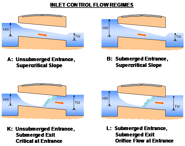
Figure 5.4: 1D Inlet Control Culvert Flow Regimes
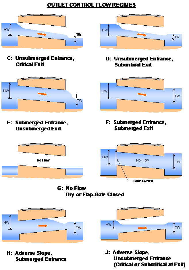
Figure 5.5: 1D Outlet Control Culvert Flow Regimes
5.7.1.1 Blockage Matrix
This feature allows for blockage of culverts to be varied based on the Average Recurrence Interval (ARI) of the flood simulation. This applies to C (circular) and R (rectangular) type culverts. For Australian users, this hydraulic structure blockage option is consistent with Project 11 of Australian Rainfall & Runoff (Weeks et al., 2013).
Two different blockage methods are available:
- The first method reduces the area in the culvert;
- The second applies a modified energy loss value to account for the blockage.
Please refer to Ollett & Syme (2016) for background information on the loss approaches.
Each culvert can be assigned a blockage category, which is defined in the 1d_nwk pBlockage attribute as a character field. A matrix of blockage category and percentage blockage for a range of ARIs is defined. Please see Section 5.7.1.1.4 for guidance on implementation.
5.7.1.1.1 Reduced Area Method
For the reduced area method, the culvert area is reduced to match the specified blockage in the same manner as varying the pBlockage attribute on the 1d_nwk layer (refer to Table 5.5). For example, with a blockage value of 10 the culvert area is reduced by 10%.
5.7.1.1.2 Energy Loss Method
For this method the area of the culvert is not modified, however, an increased entrance energy loss is applied. The modified energy loss is based on the specified culvert entry loss and the blockage ratio as per equation (5.4) (Witheridge, 2009):
\[\begin{equation} C_{ELC\_ modified} = \left( \frac{1 + \sqrt{C_{ELC}}}{BR} - 1 \right)^{2} \tag{5.4} \end{equation}\]
Where:
- \(C_{ELC\_ modified}\) = Modified culvert entry loss value
- \(C_{ELC}\) = Specified culvert entry loss value
- \(BR\) = Blockage ratio (area of blocked culvert / area unblocked culvert)
When BR is 1 (unblocked), the modified entry loss coefficient becomes the specified entry loss coefficient. The modified coefficients for a range of blockages are provided in Table 5.7.
| CELC | ||||
|---|---|---|---|---|
| 0.3 | 0.5 | 0.7 | ||
| Specified % Blockage | BR | CELC_modified | ||
| 0 | 1 | 0.3 | 0.5 | 0.7 |
| 10 | 0.9 | 0.5 | 0.8 | 1.1 |
| 25 | 0.75 | 1.1 | 1.6 | 2.1 |
| 50 | 0.5 | 4.4 | 5.8 | 7.1 |
| 75 | 0.25 | 27 | 34 | 40 |
| 90 | 0.1 | 210 | 260 | 300 |
| 95 | 0.05 | 900 | 1100 | 1280 |
| 100 | 0 | ∞ | ∞ | ∞ |
Whilst loss values of greater than 1.0 may appear counter-intuitive, it is appropriate in this situation. In conduit hydraulics there are two types of loss coefficients that are used to represent constrictions, one type being applied to the velocity at the constriction itself (these are always <=1), and the other type which are applied to the full-barrel velocity downstream of the blockage where the loss coefficient may approach infinity. The second type is convenient as the velocity downstream of the blockage is readily available and requires no manipulation of culvert geometry, and follows in principle the same application of valve coefficients. The equation above simply gives the conversion between these two types of loss coefficients.
Note: The minimum blockage ratio is set to 0.001 or 0.1%. This is required to avoid a divide by zero error in the calculations. This loss method only applies when the culvert is operating under outlet control. For an inlet control flow regime no energy loss is applied, the reduced area method is used instead.
5.7.1.1.3 Blockage Matrix Commands
The commands available for the Blockage Matrix method are listed in Table 5.8.
| Command | Description |
|---|---|
| Blockage Matrix | Turns on or off the blockage matrix functionality outlined in this section. The default is for this feature to be off. |
| Blockage Matrix File | Specifies a blockage file containing the blockage values for the various blockage categories and ARI values. |
| Blockage Method | Specifies whether to use RAM (Reduced Area Method) or ELM (Energy Loss Method). No default approach is applied. This command must be specified if using the blockage matrix functionality. |
| Blockage ARI | Specifies the ARI for the current simulation. This would typically be defined in an event file (.tef). |
| Blockage Override | Sets the blockage for all culverts with the specified blockage category. This option is useful for running simulations under an “all clear” case. |
| Blockage Default | Sets the blockage category for culverts that do not have a blockage type specified (including those that have a numeric pBlockage defined) |
| Blockage PMF ARI | If PMF has been specified in the ARI column of the blockage matrix, this command sets an ARI to be used for the PMF. This allows for interpolation of blockages for ARI values up to the PMF. |
5.7.1.1.4 Implementation
To make use of this feature the 1d_nwkb GIS layer may be used. This layer is identical to the 1d_nwk layer but the pBlockage attribute of the layer is a character field instead of a float (numeric) type. See Table 5.9. This has not been made the default field type in the 1d_nwk empty (template) files that TUFLOW produces, for two main reasons:
- A character field is bigger and less efficient to read, this could slow down simulation start-up for models not using the blockage categories; and
- A numeric field (in almost all GIS packages) defaults to 0.0, i.e. no blockage. This is not the case for a character field.
As an alternative to the 1d_nwkb GIS layer, the pBlockage attribute of the 1d_nwk GIS layer can be changed from a float (numeric) type to a character field, with maximum width of 50. Instructions on how to change the GIS layer attribute type in QGIS, ArcMap and MapInfo are provided in the TUFLOW Wiki as per the links below:
| No. | Default GIS Attribute Name | Description | Type |
|---|---|---|---|
| 1 | ID | Same as for Table 5.5. | Char(12) |
| 2 | Type | Same as for Table 5.5. | Char(4) |
| 3 | Ignore | Same as for Table 5.5. | Char(1) |
| 4 |
UCS (Use Channel Storage at nodes) |
Same as for Table 5.5. | Char(1) |
| 5 | Len_or_ANA | Same as for Table 5.5. | Float |
| 6 | n_nF_Cd | Same as for Table 5.5. | Float |
| 7 | US_Invert | Same as for Table 5.5. | Float |
| 8 | DS_Invert | Same as for Table 5.5. | Float |
| 9 | Form_Loss | Same as for Table 5.5. | Float |
| 10 | pBlockage |
C, R Channel Type: 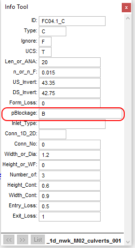
I Channel Type: |
Char(50) |
| 11 | Inlet_Type | Not used. | Char(256) |
| 12 | Conn_1D_2D | Not used. | Char(4) |
| 13 | Conn_No | Not used. | Integer |
| 14 | Width_or_Dia | Same as for Table 5.5. | Float |
| 15 | Height_or_WF | Same as for Table 5.5. | Float |
| 16 | Number_of | Same as for Table 5.5. | Integer |
| 17 | HConF_or_WC | Same as for Table 5.5. | Float |
| 18 | WConF_or_WEx | Same as for Table 5.5. | Float |
| 19 | EntryC_or_WSa | Same as for Table 5.5. | Float |
| 20 | ExitC_or_WSb | Same as for Table 5.5. | Float |
Each blockage category must be defined in the Blockage Matrix File. The first column should contain the Average Recurrence Interval (ARI) for a range of events, any additional columns contain percentage blockages for each of the ARIs. An example blockage matrix file is provided in Table 5.10 containing 5 different blockage categories (A, B, C, D, E). For blockage category A the culvert is unblocked for all ARIs, for category E the culvert is fully blocked for all ARIs. For the categories B, C, and D the blockage varies by ARI.
If the specified ARI sits between the defined ARI values in the blockage matrix file a linear interpolation is used. For example, in the table below for a 50-year ARI, blockage category “C” will have a blockage of 13.75%.
| ARI | A | B | C | D | E |
|---|---|---|---|---|---|
| 1 | 0 | 10 | 10 | 10 | 100 |
| 20 | 0 | 10 | 10 | 20 | 100 |
| 100 | 0 | 10 | 20 | 50 | 100 |
| 2000 | 0 | 20 | 50 | 70 | 100 |
| 10000 | 0 | 50 | 70 | 100 | 100 |
The ARI values for the blockage matrix file should be in ascending order. “PMF” can be defined in the ARI column, if this is done, an ARI must be assigned to the PMF using the command Blockage PMF ARI.
Example TUFLOW commands
.tcf file commands
.tef file commands
A working example of a blockage matrix model is provided in the 1D Structures Example Model Dataset on the TUFLOW Wiki.
5.7.1.2 Limitations
For the energy loss method, the loss value only applies to the culverts when flowing in outlet control flow regimes. When the flow conditions are inlet controlled TUFLOW reverts to using the reduced area method. This is required, as there is no guidance how to adjust the contraction coefficients or otherwise as used by the inlet controlled culvert equations.
5.7.2 Bridges
5.7.2.1 Bridges Overview
Bridge channels do not require data for length, Manning’s n, divergence or bed slope (they are effectively zero-length channels, although the length is used for automatically determining nodal storages – see Section 5.12.1.1). The bridge opening cross-section is described in the same manner to a normal channel.
Two types of bridge channels can be specified:
- “B” bridges require the user to specify an energy loss versus elevation table, usually derived from loss coefficients in the literature such as “Hydraulics of Bridge Waterways” (Bradley, 1978) or “Guide to Bridge Technology Part 8, Hydraulic Design of Waterway Structures” (Austroads, 2018). The energy loss table can be generated automatically via the 1d_nwk Form_Loss attribute if the energy loss coefficient is constant up to the underside of the bridge deck.
- “BB” bridges automatically calculate the form (energy) losses associated with the approach and departure flows as the water constricts and expands. It also automatically applies bridge deck losses associated with pressure flow. The only user specified loss coefficients required for BB bridges are the pier losses and the deck losses once fully submerged. If the pier loss coefficient is constant through the vertical the coefficient can simply be specified via the 1d_nwk Form_Loss attribute as described further below.
For B bridges, two bridge flow approaches are offered using Bridge Flow. Method B is an enhancement on Method A by providing better stability at shallow depths or when wetting and drying. There are also some subtle differences between the methods in how the loss coefficients are applied at the bridge deck. This is discussed further below. Method B is the approach recommended with Method A provided for legacy models. For
5.7.2.2 Bridge Cross-Section and Loss Tables
The cross-sectional shape of the bridge is specified in the same manner as for open channels using a 1d_xs GIS layer (refer to Section 5.6 and Table 5.4) and the command Read GIS Table Links. The line is digitised midway across the 1d_nwk channel line (do not specify as an end cross-section, i.e. a cross-section line snapped to an end of the bridge channel). As per the open channel, the cross-section data can be in offset-elevation (XZ) or height-width (HW) format.
Bridge structures are modelled using a height varying form or energy loss coefficient. A table (referred to as a Bridge Geometry “BG” or Loss Coefficient “LC” Table) of backwater or form loss coefficient versus height is required. The interpretation of loss coefficients provided by the user differs depending on whether the bridge channel is of a B or BB type as discussed in the following sections.
BG Tables can be entered using .csv files via a 1d_bg GIS layer (see Table 5.12) using the command Read GIS Table Links. A line is digitised crossing the 1d_nwk channel in the same manner as for the 1d_xs GIS layer used to define the cross-sectional shape of the bridge. The line does not have to be identical to the cross-section line.
Where the loss coefficient is constant through to the bridge deck (e.g. no losses such as a clear spanning bridge, or pier losses only – see BB bridges), the BG table can automatically be created by specifying a positive non-zero value for the Form_Loss attribute in the 1d_nwk layer (see Table 5.11). How the Form_Loss attribute is interpreted differs between B and BB bridge channels as discussed in the following sections.
Any wetted perimeter or Manning’s n inputs in the hydraulic properties table are ignored. If the flow is expected to overtop the bridge, a parallel weir channel should be included to represent the flow over the bridge deck, or a BW or BBW channel can be specified (see Section 5.7.4.5).
5.7.2.3 B Bridge Losses Approach
The coefficients for B bridges are usually obtained from publications such as “Hydraulics of Bridge Waterways” (Bradley, 1978) or “Guide to Bridge Technology Part 8, Hydraulic Design of Waterway Structures” (Austroads, 2018), through the following procedure.
- The bridge opening ratio (stream constriction ratio), defined in Equations 1 and 2 of “Hydraulics of Bridge Waterways” (Bradley, 1978), is estimated for various water levels from the local geometry. Alternatively, the bridge opening ratio is estimated with the help of a trial modelling run in which the stream crossed by the bridge is represented by a number of parallel channels, providing a more quantitative basis for estimating the proportion of flow obstructed by the bridge abutments.
- For each level this enables the value of Kb to be obtained from Figure 6 of “Hydraulics of Bridge Waterways” (Bradley, 1978). Additional factors, for piers (Kp from Figure 7), eccentricity (Ke from Figure 8) and for skew (Ks from Figure 10) make up the primary contributors to Kb.
- The backwater coefficient Kb input into the LC table is the sum of the relevant coefficients at each elevation. The velocity through the bridge structure used for determining the head loss is based on the flow area calculated using the water level at the downstream node.
Backwater coefficients derived in this manner have usually taken into account the effects of approach and departure velocities (via consideration of the upstream and downstream cross-section areas), in which case the losses for the B channel should be fixed. This is the default setting or can be manually specified using the “F” flag (i.e. a “BF” channel) in the 1d_nwk Type attribute, or use
For
The value of 1.5625 is derived from the following equation (5.5) presented in Waterway Design - A Guide to the Hydraulic Design of Bridges, Culverts and Floodways (Austroads, 1994):
\[\begin{equation} Q = {C_d}{b_N}Z\sqrt{2gdH} \tag{5.5} \end{equation}\]
Where:
- Q = Total discharge (m3/s or ft3/s)
- Cd = Coefficient of discharge (0.8 for a surcharged bridge deck)
- bN = Net width of waterway (m or ft)
- Z = Vertical distance under bridge to mean river bed (m or ft)
- dH = Upstream energy (or water surface) level minus downstream water surface level (m or ft)
Note: Metric (SI) units are TUFLOW’s default. To use imperial units, ensure
Assuming \({V} = \frac{Q}{b_{N}Z}\) and \(dh = K\frac{V^2}{2g}\), the equation rearranges to give \(K = \frac{1}{C_d^2}\), where a Cd value of 0.8 equates to a K energy loss value of 1.5625.
5.7.2.4 BB Bridge Losses Approach
BB bridges break down the energy losses into the following categories:
- Bridge pier losses;
- Losses due to flow contraction and expansion;
- Bridge deck losses when the bridge is submerged but not under pressure flow condition; and
- If under pressure flow, the pressure flow equation is applied as described further below.
BB bridges differ from B bridges in that the losses due to flow contraction and expansion, and the occurrence of pressure flow are handled automatically. The only loss coefficient required to be specified is that due to piers (via the Form_Loss attribute value or a LC table). Other loss parameters can be either set based on the default parameters, or can be specified by users. The parameters used by the BB bridge routine are:
- Cd = the Bridge Deck surcharge coefficient (Default = 0.8).
- DLC = the Deck loss coefficient (Default = 0.5) and only applies when no LC table exists and an automatically generated table using the 1d_nwk Form_Loss attribute is created.
- ELC = the unadjusted entry loss coefficient (Default = 0.5).
- XLC = the unadjusted exit loss coefficient (Default = 1.0).
The .ecf command “
The above values can also be changed for an individual bridge using the following 1d_nwk attributes. If the attribute value is zero then the default value or the value specified by Bridge Zero Coefficients is used.
- CD = HConF_or_WC
- DLC = WConF_or_WEx
- ELC = EntryC_or_WSa
- XLC = ExitC_or_WSb
The entrance and exit losses are adjusted every timestep according to the approach and departure velocities based on the equations below from Section 5.7.7. This approach yields similar results to the approach for determining contraction and expansion losses in publications such as “Hydraulics of Bridge Waterways” (Bradley, 1978) or “Guide to Bridge Technology Part 8, Hydraulic Design of Waterway Structures” (Austroads, 2018).
\[\begin{equation} C_{ELC\text{_}adjusted} = C_{ELC}\left\lbrack 1 - \frac{V_{approach}}{V_{structure}} \right\rbrack \tag{5.6} \end{equation}\]
\[\begin{equation} C_{XLC\text{_}adjusted} = C_{XLC}\left\lbrack 1 - \frac{V_{departure}}{V_{structure}} \right\rbrack^{2} \tag{5.7} \end{equation}\]
Where:
- V = Velocity (m/s or ft/s if using
Units == US Customary )
- C = Energy Loss Coefficient
Pressure flow is handled by transitioning from the equation described in the previous section (to derive the K value of 1.5625 from a coefficient of discharge value of 0.8) to a fully submerged situation where a deck energy loss is applied. The flux is calculated based on both the fully submerged situation and the pressure flow situation, and the lesser of the two fluxes is applied. The 1d_nwk HConF_or_WC attribute can be used to vary Cd (default value is 0.8) and the WConF_or_WEx attribute to set the submerged deck loss coefficient. When pressure flow results the “P” flag will appear in the .eof file and _TSF layer.
Optionally, LC tables can be specified for BB bridges. If a LC table exists, the Deck loss coefficient (DLC) will be ignored, while the other 3 parameters (CD, ELC and XLC) are not affected. The LC tables for BB bridges should only be the losses due to piers and bridge decks. The LC table should not include any losses for contraction, expansion and pressure flow. Note the Form_Loss value is added to the LC table loss values.
If no LC table exists for the BB bridge, and the 1d_nwk Form_Loss attribute is greater than 0.0001, a LC table is automatically generated using Form_Loss for the pier losses and the WConF_or_WEx for the Deck Loss coefficient (DLC).
Other notes are:
- BB bridges are only available if
Structure Routines == 2013 (the default).
- The unadjusted entry and exist losses (ELS and XLC) cannot be below 0 or greater than 1, and will be automatically limited to these values.
- _TSF and _TSL layers contain the following flags/values for BB bridges:
- For normal flow (“ ” or “D” if drowned out): fixed / adjusted components
- For Pressure (“P”) flow: Deck surcharge Coefficient / 0.0
- Other flags:
- “U” for upstream controlled flow – only occurs when downstream water level is below the bridge bed level.
- “Z” for zero or nearly zero flow.
- “U” for upstream controlled flow – only occurs when downstream water level is below the bridge bed level.
- For normal flow (“ ” or “D” if drowned out): fixed / adjusted components
A working example of a model containing an BB bridge is provided in the 1D Structures Example Model Dataset on the TUFLOW Wiki.
| No. | Default GIS Attribute Name | Description | Type |
|---|---|---|---|
| 1 | ID | Unique identifier up to 12 characters in length. It may contain any character except for quotes and commas, and cannot be blank. As a general rule, spaces and special characters (e.g. “\”) should be avoided, although they are accepted. The same ID can be used for a channel and a node, but no two nodes and no two channels can have the same ID. | Char(12) |
| 2 | Type | “B” or “BB” as specified in Table 5.1. | Char(4) |
| 3 | Ignore | If a “T”, “t”, “Y” or “y” is specified, the object will be ignored (T for True and Y for Yes). Any other entry, including a blank field, will treat the object as active. | Char(1) |
| 4 |
UCS (Use Channel Storage at nodes). |
If left blank or set to Yes (“Y” or “y”) or True (“T” or “t”), the storage based on the width of the channel over half the channel length is assigned to both of the two nodes connected to the channel. If set to No (“N” or “n”) or False (“F” or “f”), the channel width does not contribute to the node’s storage. See Section 5.12 for further discussion. | Char(1) |
| 5 | Len_or_ANA | Only used in determining nodal storages if the UCS attribute is set to “Y” or “T”. Not used in conveyance calculations. | Float |
| 6 | n_nF_Cd | Not used. | Float |
| 7 | US_Invert | Sets the upstream and downstream inverts. Note that the invert is taken as the maximum of the US_Invert and the DS_Invert attributes. Use -99999 to use the bed of the cross-section as the invert. | Float |
| 8 | DS_Invert | Sets the downstream invert of the channel using the same rules as for described for the US_Invert attribute above. | Float |
| 9 | Form_Loss |
If a LC table exists, for BB bridges adds the value specified to the loss coefficients in the LC table. Not added to LC tables for B bridges. If no LC table exists, and the value is greater than zero, TUFLOW automatically generates a LC table of constant loss coefficient up until the bridge deck (i.e. the top of the cross-section). The interpretation of the LC table generated from the Form_Loss value differs depending on whether a B or a BB bridge as follows: For B bridges (with no LC table):
For BB bridges (with no LC table):
|
Float |
| 10 | pBlockage | Not used. Reserved for future builds to fully or partially block B channels. The 1d_xs Skew attribute can be used to partially block cross-sections of these channels – see Table 5.4. | Float |
| 11 | Inlet_Type | Leave blank unless using the legacy MIKE 11 1D cross-section data feature. | Char(256) |
| 12 | Conn_1D_2D | Leave blank unless using the legacy MIKE 11 1D cross-section data feature, or if accessing a Flood Modeller cross-section database (.pro file), enter the label in the .pro file. | Char(4) |
| 13 | Conn_No | Leave blank unless using the legacy MIKE 11 1D cross-section data feature. | Integer |
| 14 | Width_or_Dia | Not used. | Float |
| 15 | Height_or_WF | Not used. | Float |
| 16 | Number_of | Not used. | Integer |
| 17 | HConF_or_WC |
B bridges: Not used. BB bridges: Bridge deck pressure flow contraction coefficient (Cd). If set to zero the default of 0.8 or that specified by Bridge Zero Coefficients is used. |
Float |
| 18 | WConF_or_WEx |
B bridges: Not used. BB bridges: Bridge deck energy loss coefficient (DLC) for fully submerged flow. If set to zero the default of 0.5 or that specified by Bridge Zero Coefficients is used. |
Float |
| 19 | EntryC_or_WSa |
B bridges: Not used. BB bridges: Unadjusted entrance energy loss coefficient (ELC). If set to zero the default of 0.5 or that specified by Bridge Zero Coefficients is used. |
Float |
| 20 | ExitC_or_WSb |
B bridges: Not used. BB bridges: Unadjusted exit energy loss coefficient (XLC). If set to zero the default of 1.0 or that specified by Bridge Zero Coefficients is used. |
Float |
| No. | Default GIS Attribute Name | Description | Type |
|---|---|---|---|
| 1 | Source | Filename (and path or relative path if needed) of the file containing the tabular data. Must be a comma or space delimited text file such as a .csv file. | Char(50) |
| 2 | Type | “BG” or “LC”: Bridge energy loss coefficients (second column) versus elevation (first column) for bridge structures. | Char(2) |
| 3 | Flags | No optional flags. | Char(8) |
| 4 | Column_1 |
Optional. Identifies a label in the Source file that is the header for the first column of data (ie. elevation). Values are read from the first number encountered below the label until a non-number value, blank line or end of the file is encountered. If this field is left blank, the first column of data in the Source file is used. |
Char(20) |
| 5 | Column_2 |
Optional. Identifies a label in the Source file that is in the header for the second column of data (ie. loss coefficient). If this field is left blank, the next column of data after Column_1 is used. |
Char(20) |
| 6 | Column_3 | Not used. | Char(20) |
| 7 | Column_4 | Not used. | Char(20) |
| 8 | Column_5 | Not used. | Char(20) |
| 9 | Column_6 | Not used. | Char(20) |
| 10 | Z_Increment | Not used. | Float |
| 11 | Z_Maximum | Not used. | Float |
| 12 |
Skew (in degrees) |
Not used. | Float |
5.7.3 Arch Bridge
The 2023-03 release introduced support for arch bridges as 1D channels. The approach is based on the ‘Afflux at Arch Bridges’ (HR Wallingford, 1988). Arch bridges are defined in the 1d_nwk layer as a “BArch” type. The 1d_nwk attributes specific to an arch bridge are outlined below in Table 5.13.
When an arch bridge becomes fully submerged, the actual flux through a small arch bridge opening can diverge from the flux calculated from the approach above. By default, the arch bridge approach (HR Wallingford, 1988) is still applied when water level exceeds the bridge obvert (or soffit) level. However, a transition to orifice flow condition can be optionally turned on.
The flow rate under the orifice flow condition is calculated using Equation (5.22) with the discharge coefficient (\(C_{d}\)) set via the HConF_or_WC attribute (detailed in Table 5.13). Two options are available to calculate the final discharge coefficient based on the input 1d_nwk HConF_or_WC attribute:
- A positive HConF_or_WC value can be used to set the discharge coefficient. The recommended value is 0.799.
- If a negative value is specified, the absolute of HConF_or_WC is used as a calibration factor, i.e. the discharge coefficient = abs(HConF_or_WC) * 0.799. For example, a HConF_or_WC value of -2 will adjust the discharge coefficient to 1.598.
To enable this transition, three extra attributes must be specified: a discharge coefficient (or calibration factor), lower transition distance and upper transition distance (HConF_or_WC, EntryC_or_WSa and ExitC_or_WSb attributes outlined in Table 5.13). The transition from bridge flow to orifice flow will begin at the lower transition elevation and continue linearly until the upper transition elevation is reached. From this point, the orifice flow condition is used.
A working example of a model containing an arch bridge is provided in the 1D Structures Example Model Dataset on the TUFLOW Wiki.
| No. | Default GIS Attribute Name | Description | Type |
|---|---|---|---|
| 1 | ID | Unique identifier up to 12 characters in length. It may contain any character except for quotes and commas, and cannot be blank. As a general rule, spaces and special characters (e.g. “\”) should be avoided, although they are accepted. The same ID can be used for a channel and a node, but no two nodes and no two channels can have the same ID. | Char(12) |
| 2 | Type | “BArch” as specified in Table 5.1. | Char(4) |
| 3 | Ignore | If a “T”, “t”, “Y” or “y” is specified, the object will be ignored (T for True and Y for Yes). Any other entry, including a blank field, will treat the object as active. | Char(1) |
| 4 |
UCS (Use Channel Storage at nodes). |
If left blank or set to Yes (“Y” or “y”) or True (“T” or “t”), the storage based on the width of the channel over half the channel length is assigned to both of the two nodes connected to the channel. If set to No (“N” or “n”) or False (“F” or “f”), the channel width does not contribute to the node’s storage. See Section 5.12 for further discussion. | Char(1) |
| 5 | Len_or_ANA | Only used in determining nodal storages if the UCS attribute is set to “Y” or “T”. Not used in conveyance calculations. | Float |
| 6 | n_nF_Cd | Not used. | Float |
| 7 | US_Invert | Sets the upstream and downstream inverts. Note that the invert is taken as the maximum of the US_Invert and the DS_Invert attributes. Use -99999 to use the bed of the cross-section as the invert. | Float |
| 8 | DS_Invert | Sets the downstream invert of the channel using the same rules as for described for the US_Invert attribute above. | Float |
| 9 | Form_Loss | Not used. | Float |
| 10 | pBlockage | Not used. | Float |
| 11 | Inlet_Type | The relative path to the arch properties file (must be a .csv file). See Section 5.8.1. | Char(256) |
| 12 | Conn_1D_2D | Not used. | Char(4) |
| 13 | Conn_No | Not used. | Integer |
| 14 | Width_or_Dia | Optional skew parameter. | Float |
| 15 | Height_or_WF | Optional calibration coefficient. | Float |
| 16 | Number_of | Not used. | Integer |
| 17 | HConF_or_WC |
Discharge coefficient (\(C_{d}\)) for orifice flow (see Equation (5.22)). To enable the transition to orifice flow, specify a non-zero value for this attribute.
|
Float |
| 18 | WConF_or_WEx | Not used. | Float |
| 19 | EntryC_or_WSa |
Lower transition distance for orifice flow, measured as the depth below obvert (m or ft (if using |
Float |
| 20 | ExitC_or_WSb |
Upper transition distance for orifice flow, measured as the depth above obvert (m or ft (if using The upper transition elevation must be greater than the lower transition elevation. This field is ignored if HConF_or_WC is blank. |
Float |
The .csv for the arch properties should contain the columns outlined in Table 5.14.
| Column | Description |
|---|---|
| 1 | Start chainage for arch opening. |
| 2 | End chainage for arch opening. |
| 3 | Springing level. |
| 4 | Start chainage for arch opening. |
5.7.3.1 Arch Bridge Editor
An arch bridge creator and editor tool has been developed for the QGIS TUFLOW Plugin. This tool is available from the TUFLOW Plugin Version 3.7 or later. The documentation and examples for this tool can be found on the TUFLOW Wiki Arch Bridge Editor.
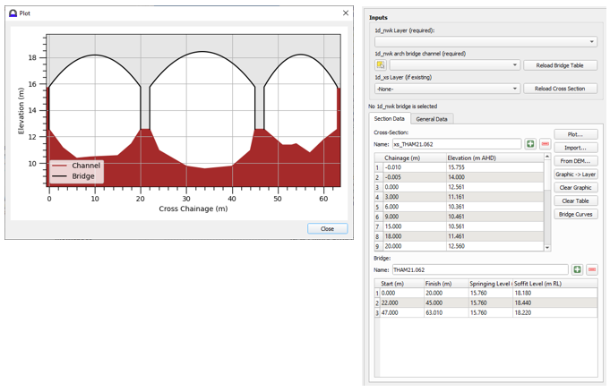
Figure 5.6: Arch Bridge Editor Tool
5.7.3.2 Arch Minimum Blockage
The flume experiments in the ‘Afflux at Arch Bridges’ (HR Wallingford, 1988) were done using medium to high bridge blockages (20%~70%), and this approach can generate extremely high velocity when the bridge blockage is close to zero percent. The 2023-03-AF release introduced a minimum blockage of 5% to stabilise the flow. This default value can be changed using the following command:
5.7.4 Weirs
5.7.4.1 Weirs Overview
A range of weir types are available as listed in Table 5.15. Weir channels do not require data for length, Manning’s n, divergence or bed slope (they are effectively zero-length channels, although the length is used for automatically determining nodal storages – see Section 5.12.1.1).
All weirs have three flow regimes of zero flow (dry), upstream controlled flow (unsubmerged) and downstream controlled flow (submerged).
| Weir Type | Description |
|---|---|
| W |
The original ESTRY weir based on the broad-crested weir formula with the Bradley submergence approach (see |
| WB | Broad-crested weir. A rectangular section shape is assumed. |
| WC | Crump weir. |
| WD | User-defined weir. |
| WO | Ogee-crested weir. |
| WR | Rectangular weir (sharp crested). |
| WT | Trapezoidal weir or Cippoletti weir. |
| WV | V-notch weir. |
| WW | Similar to the original W weir channel, but has more options allowing the user to customise the weir sub-mergence curve and other parameters. Can be based on either a rectangular shape using the 1d_nwk Width attribute or on a cross-section. |
5.7.4.2 Original Weirs (W)
For a “W” type weir, a standard weir flow formula is used as per the equation below. The weir is assumed to be broad-crested. Weirs with different characteristics should be modelled using one of the other weir types listed in Table 5.15 and discussed in Section 5.7.4.3.
\[\begin{equation} Q_{weir} = \ \frac{2}{3}CW\sqrt{\frac{2g}{C_{f}}}H^{\frac{3}{2}} \tag{5.8} \end{equation}\]
\[\begin{equation} V_{approach} = \ \frac{2}{3}C\sqrt{\frac{2gH}{C_{f}}} \tag{5.9} \end{equation}\]
Where:
- \(Q_{weir}\) = Unsubmerged flow over the weir (m3/s or ft3/s)
- \(V_{approach}\) = Velocity approaching the weir (m/s or ft/s)
- \(C\) = Broad-crested weir coefficient of 0.57
- \(W\) = Flow width (m or ft)
- \(C_{f}\) = Weir calibration factor (default of 1.0 – refer to 1d_nwk “Height_or_WF” attribute)
- \(H\) = Depth of water approaching the weir relative to the weir invert (m or ft)
Note: Metric (SI) units are TUFLOW’s default. To use imperial units, ensure
The calibration factor Cf, is available for modifying the flow. For a given approach velocity the backwater (head increment) of the weir channel is proportional to the inverse of the factor. It is normally set to 1.0 by default and modified if required for calibration or other adjustment. Note, this factor is not the weir coefficient, rather a calibration factor to adjust the standard broad-crested weir equation. The factor can be used to model other types of weirs through adjustment of the broad-crested weir equation, although use of the other weir types listed in Table 5.15 is recommended.
Huxley (2004) contains benchmarking of unsubmerged and submerged weir flow to the literature.
Note that the velocity output for a weir is the approach velocity, Vapproach, in the above equations, not the velocity at critical depth (when the flow is unsubmerged).
For submergence of W weir channels, it is recommended that Weir Approach is set to METHOD A or METHOD C. Both METHOD A and METHOD C utilises the Bradley submergence approach (METHOD C is a slight enhancement that only affects WW weir channels). The Bradley Submergence approach (Bradley, 1978), Figure 24, is handled by fitting the equation below to Bradley’s submergence curve reproduced in Figure 5.7 and applying the submergence factor to the weir equation above.
Once the percentage of submergence exceeds 70%, the submergence factor applied is given by the equation below (5.10). The Bradley curve (as digitised) and the resulting curve from the equation below are shown alongside the submergence curves used for other weir types. The submergence factor transitions the flow from weir flow to zero flow as the water level difference (dH) approaches zero.
\[\begin{equation} C_{sf} = \ 1 - \left( 1 - \frac{dH}{H} \right)^{20} \tag{5.10} \end{equation}\]
A working example of a model containing an original weir (W) is provided in the 1D Structures Example Model Dataset on the TUFLOW Wiki.
![**Bradley Weir Submergence Curve [@Bradley1978]**](images/image22.png)
Figure 5.7: Bradley Weir Submergence Curve (Bradley, 1978)
5.7.4.3 Advanced Weirs (WB, WC, WD, WO, WR, WT, WV, WW)
The advanced weirs, as listed in Table 5.15, offer greater variety, flexibility and can be customised by the user. Most of these weirs can also be operated, see Section 5.9.
The weir flow is determined by the following equation.
\[\begin{equation} Q = {\frac{2}{3}\ {\ C}_{f\ }C}_{sf}{\ C}_{d\ }W\ \sqrt{2g}{\ H}^{Ex} \tag{5.11} \end{equation}\]
Where:
- \(Q\) = Flow over the weir (m3/s or ft3/s)
- \(C_{d}\) = Weir coefficient
- \(C_{sf}\) = Weir submergence factor
- \(C_{f}\) = Weir calibration factor (default of 1.0 – refer to 1d_nwk “Height_or_WF” attribute)
- \(W\) = Flow width (m or ft)
- \(H\) = Upstream water surface or energy depth relative to the weir invert (m or ft) – see note 5 below
- \(Ex\) = Weir flow equation exponent
Note: Metric (SI) units are TUFLOW’s default. To use imperial units, ensure
Notes
- The default values for Cd are provided in Table 5.16, and documented further below for weirs where Cd is recalculated each timestep.
- The approach taken for calculating the weir submergence factor \(C_{sf}\) each timestep is documented below.
- The weir calibration factor, Cf, is by default 1.0 and should only be changed should there be a good justification.
- For weirs where the flow width (W) varies (e.g. a V-notch WV weir) the formula for that weir takes into account the varying width.
- Whether water surface depth or the energy level is used for H depends on the Structure Flow Levels setting, which can be changed on a structure by structure case using the E or H flag (see Table 5.2).
- The default values for Ex are provided in Table 5.16 .
Table 5.16 presents the weir coefficient \(C_{d}\) and weir flow exponent \(Ex\) used for each weir. Some of these values are derived from dimensional forms of the weir equations. Values other than the default values shown in Table 5.16 may be used by altering the attributes of the 1d_nwk layer. Refer to Table 5.17 for further information.
Note that \(C_{d}\) for WO and WV weirs is recalculated every timestep as described in the following sections. It is possible to override this by specifying a non-zero positive value for the “HConF_or_WC” attribute in the 1d_nwk layer. For WD weirs the user must specify a non-zero positive value.
The value for \(C_{f} \times C_{d}\) and \(C_{sf}\) is written to the TSL_P output (see Section 15.2.4) at each timestep.
The default submergence curves can be found in Figure 5.10 and Figure 5.10.
| Channel Type | Cd (HConF or WC) | Ex (WConF or WEx) | a (EntryC or WSa) | b (ExitC or WSb) | Default Submergence Curve |
|---|---|---|---|---|---|
| SP | 0.75 | 1.5 | 6.992 | 0.648 | Ogee / Nappe (Miller, 1994; USBR, 1987) |
| WB | 0.577 | 1.5 | 8.550 | 0.556 | Broad-crested from Abou Seida & Quarashi, 1976 (Miller, 1994) |
| WC | 0.508 | 1.5 | 17.870 | 0.590 | Crump H1/Hb=1.5 (Bos, 1989) |
| WD | User Defined | 1.5 | 3.000 | 0.500 | User Defined default settings |
| WO | Recalculated every timestep | 1.5 | 6.992 | 0.648 | Ogee / Nappe (Miller, 1994; USBR, 1987) |
| WR | 0.62 | 1.5 | 2.205 | 0.483 | Sharp Crest Thin Plate from Hagar, 1987a (Miller, 1994) |
| WT | 0.63 | 1.5 | 2.205 | 0.483 | Sharp Crest Thin Plate from Hagar, 1987a (Miller, 1994) |
| WV | Recalculated every timestep | 2.5 | 2.205 | 0.483 | Sharp Crest Thin Plate from Hagar, 1987a (Miller, 1994) |
| WW | 0.542 | 1.5 | 21.150 | 0.627 | Bradley 1978 Broad-crested (Bradley, 1978) |
5.7.4.3.1 Ogee Crest Weir (WO)
For WO (Ogee crest) weirs, the charts developed in USBR (1987) are used by fitting the relationship presented and plotted on the USBR curve below (Figure 5.8). The relationship falls within ±0.5% of the curve. Note that the relationship below is for US Customary Units, which is converted to metric if running the simulation in metric units. The USBR (1987) method consists of two steps:
- The ogee crest coefficient \(C_{0}\) (i.e. the discharge coefficient when the actual upstream head \(H_{e}\) = design head \(H_{0}\)) is set based on \(H_{0}\) and the height of the weir above its sill (\(P\)) as per Figure 9-23 of USBR (1987). Note that for setting the value of \(P\) the absolute difference in height between the US_Invert and DS_Invert attributes is used.
![**Ogee Spillway Discharge Coefficient, based on Figure 9-23 [@USBR1987]**](images/image24.png)
Figure 5.8: Ogee Spillway Discharge Coefficient, based on Figure 9-23 (USBR, 1987)
- When the actual head (\(H_{e}\)) is different from the design head (\(H_{0}\)) during the simulation, the discharge coefficient differs from that shown on Figure 5.8. At each simulation timestep, the discharge coefficient is adjusted based on \(H_{e}\)/\(H_{0}\) as per the chart below. The final discharge coefficient applied is \(C_{0}\) × \(C\)/\(C_{0}\) in this chart.
![**Adjustment of Discharge Coefficient based on $H_{e}$/$H_{0}$, Figure 9-24 [@USBR1987]**](images/SmallDams2.png)
Figure 5.9: Adjustment of Discharge Coefficient based on \(H_{e}\)/\(H_{0}\), Figure 9-24 (USBR, 1987)
Three options to calculate the final discharge coefficient are offered based on the input value of the 1d_nwk HConF_or_WC attribute:
- If the discharge coefficient has already been obtained by hand calculation, a positive HConF_or_WC value can be used to apply a constant discharge coefficient, i.e. \(C\) = \(C_{0}\) = HConF_or_WC.
- If the design head (\(H_0\)) is known for an ogee crest weir, a negative HConF_or_WC value can be used to specify \(H_0\). The two-step USBR (1987) method stated above will be applied to estimate the final discharge coefficient. Note this option is only available in the 2023-03-AB build or later.
- If HConF_or_WC is zero (0) or left as blank (the default), the actual head \(H_e\) at each simulation timestep will be used to estimate \(C\) from Figure 9-23 of USBR (1987), with no further adjustment based on Figure 9-24 of USBR (1987). This approach should be used when the design head (\(H_0\)) is unknown.
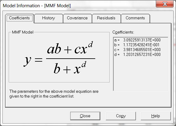
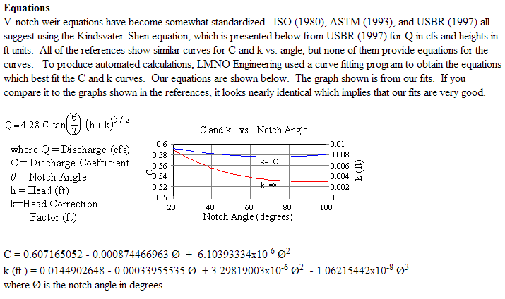
5.7.4.3.2 V-Notch Weir (WV)
For WV (V-notch) weirs, the approach taken is to use the formulae derived by LMNO Engineering as shown below. For metric models the flow is calculated in ft3/s and converted to m3/s. The top height of a V-notch weir cannot be specified, the angle continues with the increasing water level.
5.7.4.4 Advanced Weir Submergence Curves
Weir submergence factors \(C_{sf}\) were sought from two sources: “Discharge Characteristics” (Miller, 1994) and “Discharge Measurement Structures” (Bos, 1989). The submergence charts for each weir type, relating the weir submergence factor to the ratio between downstream and upstream water level were reproduced from the literature in Excel and are shown in Figure 5.10.
Two methods were utilised to fit equations to these curves. These are:
The Rational Function expressed as:
\[\begin{equation} C_{sf} = \frac{a + b\left( \frac{H_{d}}{H_{u}} \right)}{1 + c\left( \frac{H_{d}}{H_{u}} \right)\ + \ d\left( \frac{H_{d}}{H_{u}} \right)^{2}} \tag{5.12} \end{equation}\]
The Villemonte equation, expressed as:
\[\begin{equation} C_{sf} = \left( 1 - \ \left( \frac{H_{d}}{H_{u}} \right)^{a} \right)^{b} \tag{5.13} \end{equation}\]
Where:
- \(H_{u}\) = Upstream energy or water level above the weir crest (m or ft)
- \(H_{d}\) = Downstream energy or water level above the weir crest (m or ft)
- \(a, b\) = Model coefficients
Note: Metric (SI) units are TUFLOW’s default. To use imperial units, ensure
“Discharge Measurement Structures” (Bos, 1989) applies upstream energy and downstream water level to calculate \(C_{sf}\). This can be specified globally using the
For each submergence curve, the above equations were solved to obtain values for each of the variables that produced the best fit with the curves provided in the literature. After a comparison of the results, the equation from Villemonte was chosen for several reasons:
- The Rational Function was found to be sensitive to variables and required a greater number of decimal places. Villemonte was found to provide accurate results with variables requiring only 2 decimal places.
- The Villemonte equation contains only two variables, compared to four used in the Rational Function, making it simpler and less susceptible to error.
- The Villemonte equation may be solved exactly at the extremities of the curves (i.e. where \(\frac{H_{d}}{H_{u}} = \ 1\) and \(C_{sf} = 0\), and when \(\frac{H_{d}}{H_{u}}\) = 0 and \(C_{sf} = 1\)). The Rational Function required further manipulation through inclusion of additional points to achieve this outcome.
The default variables a and b used to determine the submergence factor \(C_{sf}\) for each weir type are presented in Table 5.16. Figure 5.11 shows the submergence curves produced using the default values in Table 5.16 to calculate \({\ C}_{sf}\).
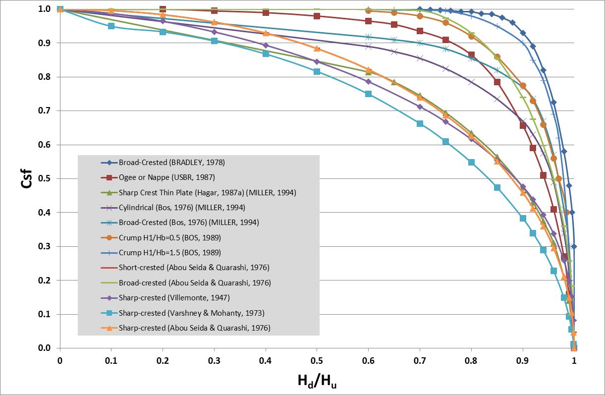
Figure 5.10: Weir Submergence Curves from the Literature
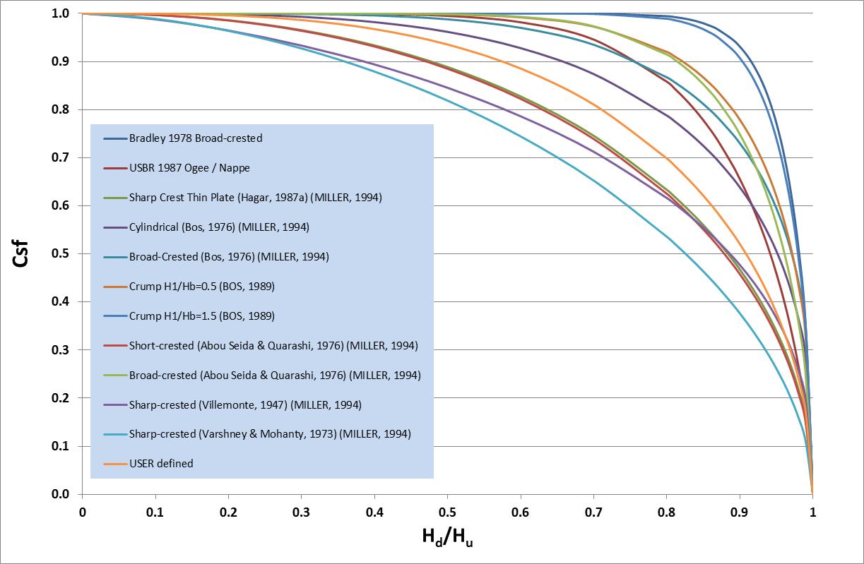
Figure 5.11: Weir Submergence Curves using Villemonte Equation
| No. | Default GIS Attribute Name | Description | Type |
|---|---|---|---|
| 1 | ID | Unique identifier up to 12 characters in length. It may contain any character except for quotes and commas, and cannot be blank. As a general rule, spaces and special characters (e.g. “\”) should be avoided, although they are accepted. The same ID can be used for a channel and a node, but no two nodes and no two channels can have the same ID. | Char(12) |
| 2 | Type | The weir channel type as specified using the flags in Table 5.1 and 5.15. For example, a V-notch weir would be entered as “WV”. | Char(4) |
| 3 | Ignore | If a “T”, “t”, “Y” or “y” is specified, the object will be ignored (T for True and Y for Yes). Any other entry, including a blank field, will treat the object as active. | Char(1) |
| 4 |
UCS (Use Channel Storage at nodes) |
If left blank or set to Yes (“Y” or “y”) or True (“T” or “t”), the storage based on the width of the channel over half the channel length is assigned to both of the two nodes connected to the channel. If set to No (“N” or “n”) or False (“F” or “f”), the channel width does not contribute to the node’s storage. See Section 5.12.1.1 for further discussion. | Char(1) |
| 5 | Len_or_ANA | The length of the weir channel, not the weir crest. Only used for automatically determining the storage at the nodes if the UCS attribute is set to “Y” or “T”. Not used in the conveyance calculations. If a no attribute is specified, the length of the digitised line is used. | Float |
| 6 | n_nF_Cd | Not used. | Float |
| 7 | US_Invert |
All Weir (excluding WO) Channel Types: The absolute difference in height between the US_Invert and DS_Invert is used to set the height of the weir above its sill (usually denoted as P), which is used for recalculating the weir’s discharge coefficient each timestep. If the US_Invert and DS_Invert are the same value the primary upstream channel bed will be used to set the value of P. |
Float |
| 8 | DS_Invert | See comments above for US_Invert. | Float |
| 9 | Form_Loss | Not used. | Float |
| 10 | pBlockage |
W Channel Type: WB, WC, WD, WO, WR, and WS Channel Type: WT Channel Type: The V-notch angle is adjusted proportionally by the % blockage. |
Float |
| 11 | Inlet_Type | Leave blank unless using the legacy MIKE 11 1D cross-section data feature. | Char(256) |
| 12 | Conn_1D_2D | Leave blank unless using the legacy MIKE 11 1D cross-section data feature, or if accessing a Flood Modeller cross-section database (.pro file), enter the label in the .pro file. | Char(4) |
| 13 | Conn_No | Leave blank unless using the legacy MIKE 11 1D cross-section data feature. | Integer |
| 14 | Width_or_Dia |
All Weir (excluding WT and WV) Channel Types: Note: For W and WW weirs if a cross-section for the channel exists, the cross-section profile will prevail over the automatic rectangular shape. Note: For operational weirs, the width of the weir when fully open. WT Channel Type: Angle of the V-notch in degrees. Must be between 20º and 100º. |
Float |
| 15 | Height_or_WF |
For non-operated weirs, this value can be used as a weir coefficient adjustment factor to be primarily used for model calibration or sensitivity testing. The weir coefficient is multiplied by this value. The resulting weir coefficient can be viewed in the .eof file and over time in the _TSL GIS layer. If zero or negative an adjustment factor of 1.0 (i.e. no adjustment) is applied. For operational weirs, the height of the weir above the crest when fully up. |
Float |
| 16 | Number_of | Not used. | Integer |
| 17 | HConF_or_WC |
W Channel Type: All Weir (excluding W) Channel Types: Note that for WV weirs the default is to recalculate Cd every timestep. Entering a value greater than zero (0) will override this and apply a fixed Cd. For WO weirs, the default is to recalculate Cd every timestep based on the actual head, while entering a value less than zero (0) will specify a design head for Cd calulation. Entering a value greater than zero (0) will apply a fixed Cd. Please see Section 5.7.4.3.1 for the detailed ogee crest weir approach. For WD weirs the user must specify a non-zero positive value. Note that published weir coefficients may be based on other non-dimensional or dimensional forms of the weir equation, and care should be taken in ensuring the coefficient is compatible with the form of the weir flow equation presented in Section 5.7.4.3. |
Float |
| 18 | WConF_or_WEx |
W Channel Type: Weir flow equation exponent Ex in the weir flow equation presented in Section 5.7.4.3. If less than or equal to zero the default value for the weir type in Table 5.16 is used. The default value is 1.5 for all weir types except for WV which is 2.5. |
Float |
| 19 | EntryC_or_WSa |
W Channel Type: Sets the submergence factor “a” exponent in the Villemonte Equation for calculating the weir submergence factor Csf (refer to equations in Section 5.7.4.3 and 5.7.4.4). If less than or equal to zero the default value for the weir type in Table 5.16 is used. |
Float |
| 20 | ExitC_or_WSb |
W Channel Type: Sets the submergence factor “b” exponent in the Villemonte Equation for calculating the weir submergence factor Csf (refer to equations in Section 5.7.4.3 and 5.7.4.4). If less than or equal to zero the default value for the weir type in Table 5.16 is used. |
Float |
5.7.4.5 Automatically Created Weirs
Weirs representing overtopping of structures such as culverts and bridges may be automatically created without the need to digitise a separate line within a 1d_nwk layer. The structure must be digitised within a 1d_nwke layer (as opposed to a 1d_nwk layer) and a “W” specified alongside the original structure type. For example, to model a bridge and a weir representing overtopping of the road deck, specify type “BW”. The weir crest level and dimensions are specified within the additional attributes contained within a 1d_nwke layer and are explained in Table 5.18. The original W weir approach is adopted for calculating the flow (see Section 5.7.4.2).
The weir’s shape is assumed to be two rectangles on top of each other. The lower rectangle is reduced in width according to the percent blockage applied to the rail (i.e. the EN4 attribute in Table 5.18), and its height is the EN3 attribute. The upper rectangle is the full flow width and extends indefinitely in the vertical.
Alternatively, the flow over a structure can be manually digitised as a separate 1d_nwk weir channel parallel to the original bridge or culvert structure (i.e. the weir is connected to the ends of the bridge/culvert). Any of the available weir types can be used in this instance.
| No. | Default GIS Attribute Name | Description | Type |
|---|---|---|---|
| 21 | ES1 | Not yet used (leave blank). | Char(50) |
| 22 | ES2 | Not yet used (leave blank). | Char(50) |
| 23 | EN1 |
For BW, CW and RW channels, the flow width of weir (m or ft (if using |
Float |
| 24 | EN2 |
For BW, CW and RW channels, the depth (m or ft (if using |
Float |
| 25 | EN3 |
For BW, CW and RW channels, the depth of the hand rail (m or ft (if using |
Float |
| 26 | EN4 | For BW, CW and RW channels, % blockage of the rail (e.g. 100 for solid rail, 50 for partially blocked, 0 for no rail). | Float |
| 27 | EN5 | For BW, CW and RW channels, the weir calibration factor. Is set to 1.0 if < 0.001 is specified. | Float |
| 28 | EN6 | Not yet used (leave as zero). | Float |
| 29 | EN7 | Not yet used (leave as zero). | Float |
| 30 | EN8 | Not yet used (leave as zero). | Float |
5.7.4.6 VW Channels (Variable Geometry Weir)
The VW (variable weir) channel allows the modeller to vary the cross-section geometry of a W weir over time using a trapezoidal shape. To set up a VW channel follow the steps below.
In the 1d_nwk layer, the following attributes are required:
- ID = ID of the channel;
- Type = “VW”;
- Len_or_ANA = Nominal length in m (only used for calculating nodal storage if UCS is on);
- US_Invert = -99999 (the invert level is specified in the .csv file discussed below);
- DS_Invert = -99999 (the invert level is specified in the .csv file discussed below);
- Inlet_Type = relative path to a .csv file containing information on how the weir geometry varies; and
- Height_Cont = Trigger Value (the upstream water level to trigger the start of the failure; upstream water level is determined as the higher water level of the upstream and downstream nodes).
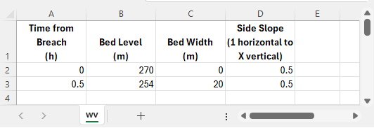
The .csv file must be structured as follows (also see example below):
- TUFLOW searches through the sheet until more than 4 numbers are found at the beginning of a row (Row 2 in the example below).
- Each row of values is read until the end of the file or a row with no or less than four numbers is found. There is no limit on the number of rows of data.
- The four columns must be as follows and in this order. The labels for the columns are optional.
- Time from start of breach in hours.
- Weir bed level in metres.
- Weir bed width in metres.
- Side slope (enter as the vertical distance in metres for one metre horizontal). For example, a value of 0.5 means a slope of two horizontal to one vertical.
- Time from start of breach in hours.
In the example below, the weir once triggered will erode from a bed level of 270m to 254m, widen from a bed width of 0 to 20m and the side slope will remain constant at 0.5. The period of time for the erosion is 0.5hours.
Although in most cases the weir is eroded, the weir can also be raised/accreted as well or a combination of the two. Simply enter the change over time using as many rows as needed.
The original W weir approach is adopted for calculating the flow (see Section 5.7.4.2).
5.7.5 Spillways (SP)
Spillways (‘SP’) were introduced for the TUFLOW 2013-12 release and may also be used in operational mode as a gated spillway (see Section 5.9). Spillways may also be simulated and operated as Q or QO channels where the user provides the stage discharge relationships (see Section 5.8.2 and Section 5.9.3). The 1d_nwk attributes are presented in Table 5.19.
Spillways use the same equation as for advanced weirs (Section 5.7.4.3). For ungated spillways (i.e. SP, non-operated spillways) the same parameters as for Ogee Weirs are the default (see Table 5.16), except for Cd, which is fixed with the default value of 0.75. For Ogee Weirs, Cd is recalculated every timestep (see Section 5.7.4.3.1). The 1d_nwk attributes in Table 5.16 can be used to modify the flow equation parameters for SP channels in a similar manner for advanced weirs.
SPO channels also use the same equation when the gate is not affecting the flow (for more information on SPO channels refer to Section 5.9.6).
SP and SPO channels can also drown out as per the submergence curves for advanced weirs.
A working example of a model containing a spillway is provided in the 1D Structures Example Model Dataset on the TUFLOW Wiki.
5.7.6 Sluice Gates (SG)
For sluice gates refer to Section 5.9.5. The same approach applies as for SGO operated gates, except that the gate is assumed to be in a fixed position based on the 1d_nwk Height_or_WF attribute value. The 1d_nwk attributes are presented in Table 5.19.
5.7.7 Adjustment of Contraction and Expansion Losses
The energy losses associated with the contraction and expansion of flow lines into and out of a structure, can be automatically adjusted according to the approach and departure velocities in the upstream and downstream channels. This is particularly important where:
- There is no change in velocity magnitude and direction as water flows through a structure. In this situation, there is effectively no entrance (contraction) or exit (expansion) losses and the losses need to be reduced to zero. Examples are:
- A clear spanning bridge over a stormwater channel where there are no losses due to any obstruction to flow until the bridge deck becomes surcharged.
- Flow from one pipe to another where the pipe size remains unchanged and there is no significant bend or change in grade.
- A clear spanning bridge over a stormwater channel where there are no losses due to any obstruction to flow until the bridge deck becomes surcharged.
- There is a change in velocity, but the change does not warrant application of the full entrance and exit loss. This is the most common case where the application of the full entrance and exit loss coefficients (typically 0.5 and 1.0) will overestimate the energy loss through the structure. The full values are only representative of the situation where the approach and departure velocities are close to zero, for example, a culvert discharging from a lake into another lake where the velocity transitions from still water to fast flowing and to still water.
The entrance and exit losses are adjusted according to the equations below to take into account the change in velocity caused by the structure. The first equation is empirical, while the second equation to adjust exit losses can be derived from first principles.
\[\begin{equation} \text{C}_{\text{entrance_adjusted}} = \text{C}_{\text{entrance}}\left\lbrack 1 - \frac{\text{V}_{\text{approach}}}{\text{V}_{\text{structure}}} \right\rbrack \tag{5.14} \end{equation}\]
\[\begin{equation} \text{C}_{\text{exit_adjusted}} = \text{C}_{\text{exit}}\left\lbrack 1 - \frac{\text{V}_{\text{departure}}}{\text{V}_{\text{structure}}} \right\rbrack^{2} \tag{5.15} \end{equation}\]
Where:
- V = Velocity (m/s or ft/s if using
Units == US Customary )
- C = Energy Loss Coefficient
As the structure velocity approaches the incoming and/or outgoing velocities, the loss coefficient approaches zero. When the incoming and/or outgoing velocity approaches zero (i.e. water is leaving/entering a large body of water), the loss coefficients approach their full value.
Tullis & Robinson (2008) provide an excellent proof for the need to adjust losses for different flow regimes using the exit loss equation above. The paper benchmarks different exit loss equations used within the industry methods against experimental flume test results.
The adjustment of losses feature is available to structures that require entrance and exit loss coefficients, namely culverts and bridges. For culverts, the adjusted entrance loss coefficient only applies where the flow is not inlet controlled (i.e. Regimes C, D, E, F, H and J in Table 5.6), and the adjusted exit loss is only influential where the flow is downstream controlled (i.e. Regimes D, F, H and J (subcritical at exit) in Table 5.6). For bridges, the application varies as discussed below.
If
For BB bridges, the LC table should only represent the pier and submerged deck losses (see Section 5.7.4.4), as the adjustment of entrance and exit losses every timestep as per the equations above is always applied irrespective of the Structure Losses setting. The equations above conform with the approach for determining contraction and expansion losses in publications such as Hydraulics of Bridge Waterways.
For B bridges and culverts, if Structure Losses is set to “ADJUST”, or “A” has been specified in the 1d_nwk Type attribute (e.g. BA, CA, IA or RA), the entrance and exit losses are adjusted according to the equations above. For B bridges, because the entrance and exit losses are combined as one loss coefficient, the entrance and exit loss components are proportioned one-third / two-thirds respectively when applying the above equations. For the new BB bridge, entrance and exit losses are always adjusted as per the equations above and the Structure Losses setting is not relevant (also see Section 5.7.4.4).
The selection of the upstream and downstream channels on which to base the approach and departure velocities is as follows:
- The upstream channel is determined as the channel which has a positive flow direction into the structure whose invert is closest to that of the upstream invert of the structure. If no channel exists, no adjustment of losses is made (this includes structures connected to a 2D domain). Note that the upstream channel must be digitised so that it has the same positive flow direction to that of the structure.
- The downstream channel is selected on a similar basis to that for the upstream channel.
- The selected upstream and downstream channels are listed in the .eof file for cross-checking (search for “Primary Channel”).
- X channels can be used to connect additional channels and ensure that these are not considered the primary channel.
TUFLOW has no requirement of a minimum loss coefficient value for stability, and allows the adjusted coefficient to approach zero allowing this feature to correctly model the structure losses when the structure causes no disturbance to flow, or when one pipe discharges into another of identical size, grade and alignment.
The adjustment of loss coefficients does not apply to:
- Any bend or additional loss for a culvert entered using the Form_Loss attribute in the 1d_nwk layer. This coefficient can be used to apply additional losses (e.g. pit or bend losses) that are not affected by changes in the relativity of the approach/departure and structure velocities.
- Any additional loss coefficient component for BB bridges entered using the Form_Loss attribute in the 1d_nwk layer. This coefficient can be used to apply additional losses (e.g. pier losses) that are not affected by changes in the relativity of the approach/departure and structure velocities.
- The ends of culverts and bridges that are connected to 2D SX or HX cells as the approach or departure velocity needs to be derived in some manner from the 2D velocity field. It is important not to be duplicating energy losses by applying exit losses to a 1D structure and simulating the same energy losses due to the flow expansion in the 2D domain – for further information see the Modelling Energy Losses at Structures AWS Webinar.
If Structure Losses is set to FIX, or “F” has been specified in the 1d_nwk Type attribute (e.g. BF, CF, IF or RF), the entrance and exit loss coefficients for B bridges and culverts are not adjusted. Fixing the entrance and exit losses for BB bridges is not available – use a B bridge instead.
Note that the energy loss specified via the “Form_Loss” attribute is not subject to this adjustment.
The variation in time of the loss coefficients can be viewed using the _TSL output layer (see Section 15.2.4) or charted in the QGIS TUFLOW Viewer plugin.
If there is a manhole at the culvert end, a manhole energy loss approach (see Section 5.10.4) is used instead of the culvert’s contraction/expansion loss, and the above description does not apply.