16.2 Troubleshooting

Despite the best efforts of a modeller to be proactive in creating healthy models, some aspect of review and troubleshooting may be required to generate a healthy and robust model.

The most common cause for an unhealthy model is poor underlying topography. In the case of 2D domains, the quality of the Digital Terrain Model (DTM) is often the problem, and investing time to create truly representative, well-constructed, DTMs is highly recommended from both the modelling perspective and the quality of the inundation mapping.

For 1D domains, topographic inaccuracies in cross-section data and at structures is often the source of problems, although model schematisation can sometime also be the source of issues. As a general statement, 1D modelling is more of an “art” than 2D modelling, due to the need for user judgement associated with the selection of cross-section locations, and schematisation of the 1D domain.

For 1D-2D models, often poor stability of the 1D domain can lead to instabilities in the combined model at higher flows when flow comes out of bank. It is suggested that the 1D model is tested to ensure stability prior to coupling with the 2D domain where possible. Care should also be taken in the schematisation of any 1D-2D linkages.

Tip: Take an iterative approach to solving problems. As a model stability issue may cascade to cause others, when searching through the _messages GIS file, resolve the problems in order of occurrence (i.e. in the order the messages appear in a QGIS attributes table, top to bottom). Solving issues earlier may automatically resolve the errors reported later in the simulation

16.2.1 General Comments

When building a model, be proactive about ensuring the data is as complete as possible and accurately reflects reality. For 1D stormwater pipe network data, use the 1D Integrity Tool is recommended to ensure data is consistent and free of common errors, prior to use within a TUFLOW model simulation. The TUFLOW ‘test’ mode can also be used to test the data inputs without the simulation phase, see Section 13.4.2.1 for more details. This can be used in the initial model testing phase without using the high specification modelling hardware that is often required for the hydrodynamic simulation.

Problems in the input data that get through this initial integrity check are readily identified by using Write Check Files command in the .tcf file and/or Write Check Files in the .ecf file to generate GIS check files. These files represent the final combination of the 2D and 1D data inputs, and are excellent for identifying data input problems. A detailed description of all available check files is provided in the TUFLOW Wiki Check Files page.

If the model becomes unstable, TUFLOW writes output data for the last computed timestep. The location of stability is easily found by viewing the results for the last timestep. Very large velocity vectors and/or excessively high or low water levels usually occur in the vicinity of the instability.The instability can also be located using the _messages.shp / .gpkg files (see Section 14.4.5).

Always search the .tlf files for the terms, “UNSTABLE”, “WARNING”, “CHECK” and “ERROR”. ERRORs stop the simulation, while WARNINGs and CHECKs do not. Note, it is possible that latter errors are caused by earlier warnings, and search through the .tlf files, or start at the beginning of the attributes within the _messages.shp/.gpkg file, resolve the earlier errors first, rather than working backwards from the final error which resulted in the instability.

The Troubleshooting section of the TUFLOW Wiki TUFLOW Messages page contains a comprehensive database of TUFLOW “CHECK”, “WARNING” and “ERROR” messages. Each “CHECK”, “WARNING” and “ERROR” message has its own Wiki page documenting a description of the message, and suggestions how to address the message.

16.2.2 Instability Identification

Instabilities usually start with one or a few computational points “bouncing” as a result of poor convergence of the mathematical equations being solved. To help identify the start of an instability, negative depth warnings are issued if the depth in a 2D cell (usually TUFLOW Classic only) or a 1D node falls below ‑0.1m. Negative depth warnings are usually a pre-cursor to an instability of the true expected solution. It is not uncommon, particularly in areas of rapid wetting and drying for negative depths to occur before the computational point is made dry (inactive). Hence a buffer of -0.1m is used before reporting a WARNING.

The WARNING messages are sent to the _messages.shp / .gpkg file (see Section 14.4.5). Import or open this file in GIS software to identify the location of the negative depth calculation. If the number of these warnings are substantial (e.g. if a model remains stable but with minor instabilities), select some of the first negative depth warnings in the attribute data and display just those. The warnings are in order of occurrence. By tracing through the negative depth warnings in the vicinity of the instability, the original source of the instability can usually be located.

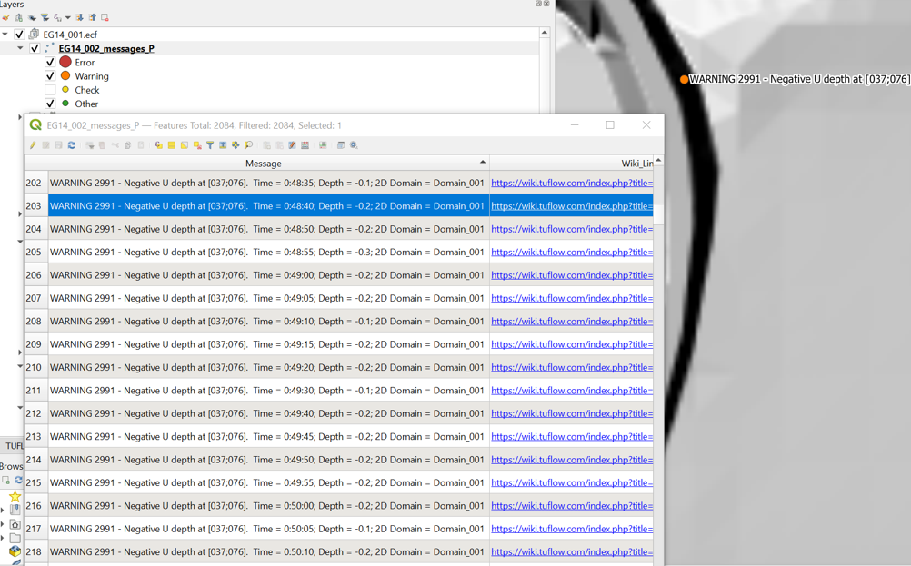
Figure 16.4: TUFLOW Warning 2551 Messages in QGIS

TUFLOW also uses defined 1D and 2D water level threshold values to trigger an instability message. The commands associated with these thresholds are Depth Limit Factor (1D domains) and Instability Water Level (2D domains).

16.2.2.1 1D (ESTRY) Domains

As advised in Section 16.2.2 for 2D domains, the location of an instability should be determined by investigating where the WARNING 1991 messages occur. Common options for helping resolve unstable or problematic 1D nodes and channels are:

If a 1D node or channel has become unstable, causing a simulation to crash yet the water levels appear stable in the results, check the Depth Limit Factor setting. It may be that the water level is simply exceeding the maximum depth of the node/channel times the Depth Limit Factor.
If a 1D node has repeated WARNING 1991 messages, and/or has a mass error problem, check that the cross-section/structure dimensions of adjoining channels are correct and appropriate. Common causes are:
1. A large change in cross-sectional area for successive channels. If the channel is natural, then it is likely that one or more of the cross-sections are not representative of the real situation.
2. One or more incorrect upstream and downstream bed levels. Import the 1d_inverts_check GIS file, label the Invert attribute, and cross-check that the inverts are correct.
3. A very steep channel entering a gently sloping channel. If this is the real situation, then additional 1D channels providing a higher computational resolution may be needed, alternatively inserting a structure at the transition may help.
4. If there is a sudden change in 1D flow area, then a more appropriate and more stable approach would be to insert a structure representative of the situation to model the energy losses associated with the contraction and/or expansion of the water.
5. Trial using a smaller 1D Timestep to establish whether the problem is timestep related. If it is not timestep related, reducing the timestep should have little change in results. In some problematic models, 1D instabilities may actually magnify with a reducing timestep.
6. A common solution is to add additional storage to the 1D node. This can be done by using the 1d_nwk Length_or_ANA attribute described in Table 5.31 or using Minimum NA, Storage Above Structure Obvert or Minimum Channel Storage Length. Usually adding additional storage at problematic nodes does not adversely affect the results (unless there are a lot of problematic nodes), however, this should be checked through sensitivity testing (this can be carried out by adding even more storage again and ascertaining the effect on the hydraulic results).

Besides investigating where the WARNING 1991 messages occur, the most effective approach to identify potential problem locations is to thematically map or categorise the _TSMB GIS layer using the ME_Avg_Abs attribute.

16.2.2.2 TUFLOW Classic

To identify problematic areas within a TUFLOW Classic 2D domain, the most common approach is to run the model at a reasonable timestep and investigate where the WARNING 2991 messages occur. If mass error is an issue in the 2D domain, the MB1 and MB2 outputs (see Map Output Data Types and Table 11.4 may be of use.

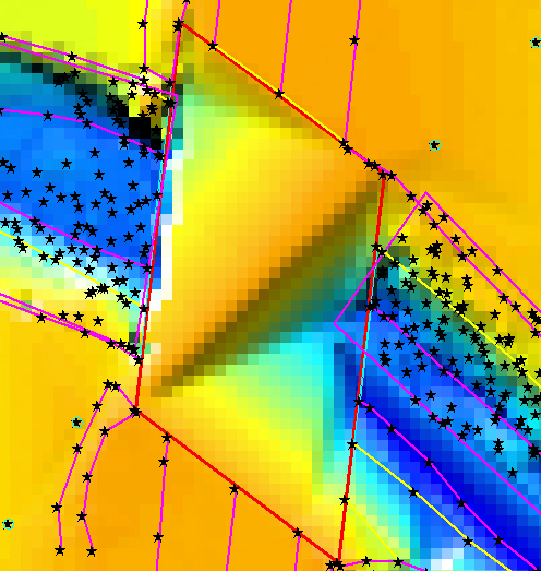
Of particular note, models based on high quality DTMs are as-a-rule rarely problematic. However, if the DTM is rough or “bumpy” (as can be the case with air-borne laser DTMs), or has poor triangulation causing sharp ridges as illustrated in the images below, models based on these DTMs are much more likely to be problematic in/near these areas.

The following steps are useful to help identify and resolve the problem.

Set the 2D Timestep to somewhere between \(\frac{1}{2}\) to \(\frac{1}{5}\) of the cell size (in metres).
Run the model until it becomes unstable or has generated the WARNING 2991 messages.
Import or open the _messages GIS layer.
Within your chosen GIS package, view the _messages GIS layer in a tabular format and try to trace back from the “UNSTABLE 2999” messages to the initial “WARNING 2991” messages that were most likely the trigger for the instability.
Select a few of these WARNINGs and locate them geographically in the GIS map window.
Using the various _check GIS layers, carry out some fundamental checks. For example:
1. 2d_zpt_check or _DEM_Z check file: Check the Zpt values are as you would expect. If the Zpt values are particularly “bumpy”, try smoothing the ones at/near the WARNING 2991 messages. Where the Zpts change in elevation rapidly (e.g. the outside bend of a river), deep ZU and ZV elevations can be problematic. If modifying the ZU and ZV values, tend to assign an elevation closer to the higher of the two ZC values either side of the ZU/ZV point. To modify the Zpts it is recommended to create a new 2d_zpt or 2d_zsh layer rather than editing the original data source for quality control purposes.
2. 2d_uvpt_check or 2d_grd_check: check the Manning’s n values are as expected, if not identify why.

For reference, a detailed description of all available check files is provided in the TUFLOW Wiki Check Files page.

Other points to note for TUFLOW Classic 2D domains are:

If the model becomes unstable quickly and the instability location is near a 2D water level boundary, check that the initial water level setting is compatible with the starting water level of the boundary.
Direct rainfall modelling on high elevations(>100m) may experience unacceptable mass errors due to a floating point imprecision problem. These models need to use the double precision version of TUFLOW (see Section 13.3.2). In addition, the default Cell Wet/Dry Depth may need to be lowered from 0.002m to 0.0002m (when using Units == US Customary the equivalent would be lowering from the default of 0.007 to 0.0007ft) due to the substantial amount of sheet flow.

16.2.2.3 TUFLOW HPC

To identify problematic areas within a TUFLOW HPC 2D domain, the most common approach is to output the ‘dt’ map output (see Map Output Data Types and Table 11.4), and identify the locations where the lowest timestep (dt) values occur (see Figure 16.1). For those locations, check files are reviewed to search for data input issues. Of the check files, possibly the most useful for TUFLOW HPC is the _DEM_Z check file in the location of the _dt_min to assess the topography representation. If the topography doesn’t look realistic, it’s useful to open the zsh_zpt_check file to assess if there’s any topographic modifications made in this location, or whether there is an artefact in the input DTM datasets that is causing the irregularity. The TUFLOW styles can be applied to the zsh_zpt_check file check file to show different adjustments, red upwards arrows for increased elevation values, blue downwards arrows for decreased elevation values.

Other points to note for TUFLOW HPC 2D domains are:

Non-perpendicular boundaries can provide instabilities in both TUFLOW Classic and HPC. Whereas in TUFLOW Classic they will likely lead to an unstable model, they are more challenging to pick up with TUFLOW HPC because of its unconditionally stability. One approach to review inflow boundaries in a TUFLOW HPC model is to a add 2d_po line immediately downstream of any boundary inputs. The PO results can then be used for detailed review of the model stability in that particular location.
TUFLOW HPC simulates flow depth as its state variable and it does not suffer the same potential loss of precision as TUFLOW Classic when modelling direct rainfall. It is not a requirement to run a double precision version of TUFLOW HPC for direct rainfall applications. There are some situations in which TUFLOW HPC may benefit from double precision, for more information see Section 13.3.2.2.

16.2.2.4 1D/2D Links

Some common configuration mistakes associated with 1D/2D links, and recommendations to resolve them are:

Using a mixture of connected HX and SX lines along a river bank can cause mass errors. This is not a recommended configuration. In these situations the 1D and 2D mass error reporting can appear satisfactory, however the overall model mass error is poor. HX connections are the recommended configuration to connect the 1D open channel to the 2D representation of the floodplain. The _TSMB1d2d GIS layer is useful for identifying mass error issues across 2D HX lines. Note, the units of the mass error values for this layer are presently in m³s^-1, not in percent.
Unrealistic flow patterns occurring across the HX lines, sometimes causing strange flow patterns and circulations in the 2D domain. This behaviour may occur due to one of the following reasons:
1. Insufficient spatial resolution in the 1D domain. If the interval between 1D nodes is too large, then the linearly interpolated 1D water level profile that is transferred from the 1D domain to the 2D domain along the HX line will not accurately reflect the real situation. This can create recirculation in the 2D and oscillations in the 1D. Check that there is a sufficiently fine resolution of 1D nodes along the river to be representative of the river’s longitudinal water surface slope. Typically, areas where there are significant changes in longitudinal water surface gradient will require finer 1D resolution. Additional 1D nodes may be incorporated quickly and easily in the model through the use of automatically interpolated cross-sections (refer to Section 5.6.7).
2. Conversely, having too fine a spatial 1D resolution may cause stability problems due to insufficient nodal storage. As a general rule-of-thumb, the node surface area should be similar to the width of the 1D/2D interface multiplied by 3 to 10 cell widths.
3. At a junction of three or more 1D channels, care should be exercised in how the levels from the side branches are transferred to the HX line(s). If the side branch has much higher water levels than the main branch, and a HX line segment is connected at one end to the side branch and the other end to the main branch, a steep water level gradient may be applied along the HX line segment that is not particularly representative of the real situation.
4. Similarly, at 1D structures where there is a significant drop in water level (for example, across a weir), the HX line may need to be stopped upstream and restarted downstream of the structure to prevent a steep gradient being applied across HX cells over the structure.
Instabilities can occur across HX boundaries that are located in areas of ponding water due to the frequent transfer of water back and forth between the 1D and 2D domains. Use the 1D_2D_check layer to view the ZC elevations of the boundary, ensuring the elevations are appropriate and the boundaries have been digitised on the top of banks. In some situations the HX boundaries may need to be relocated and the schematisation of the model revisited to resolve the issue.
Bumpy topography in the approach to SX boundaries may lead to instabilities. Smooth out the Zpt elevations where appropriate, ensuring there is a 2D flow path leading to / departing from the boundary.
An inappropriate number of SX boundary cells in relation to the 1D structure width may cause stability problems. The number of cells selected should generally always correlate to the 1D structure width. For example, a 5m wide culvert should be connected to 2-3 SX boundary cells when the cell size is 2m wide. If the 1D structure width is less than or equal to a single cell width, two rather than one boundary cell may need to be selected to achieve stability.

16.2.2.5 Other General Troubleshooting Recommendations

Futher general suggestions for common situations that are not uniquely specific to TUFLOW 1D, Classic, HPC or 1D/2D linking are provided below.

If the Console Window does not appear at all when executing a simulation, check for virtual memory congestion (see Section 14.1.3).
If the Console Window disappears for no apparent reason, first check the following:
1. You have sufficient disk space on the drive you are writing your results to and where the .tcf or .ecf files are located (this is where the .tlf file is written by default).
2. Your computer network is/was not down.
3. If you are executing TUFLOW from a Windows batch file, review the batch file syntax is correct.
If TUFLOW indicates that GIS objects are not snapped, not connected, could not be found or are outside the model domain, check that:
1. The most recent GIS updates have been saved or exported for use by TUFLOW.
2. The relevant GIS layers are in the correct projection and that the objects are snapped to each other. Some GIS programs can handle layers of different projections, however, TUFLOW requires that all layers be in the same projection. This projection must be a Cartesian projection (not degrees latitude/longitude) and is specified using SHP Projection, GPKG Projection and/or MI Projection in the .tcf file. The default setting is that all input layers are of the same projection otherwise an ERROR occurs (see GIS Projection Check).
3. Different GIS software may use a different precision in the coordinates, this may result in objects being snapped within the software but not in TUFLOW. The distance which objects are considered snapped in TUFLOW can be set with the Snap Tolerance command in TUFLOW.
If you are experiencing instability water levels. Follow the advice given in Section 16.2.2 and 16.2.2.1. Otherwise, check the water level that is used for detecting instabilities (Instability Water Level). If every Z point elevation has not been allocated, the default elevation of 99999 will be assigned. Provided the default settings for the .tcf command Zpt Range Check have not been altered, TUFLOW will report an ERROR message. If there are very high Z points in your geometry (relative to your water levels), this allows any instabilities to oscillate in a very large range. Consequently, the instability can become so extreme that floating point errors (i.e. the computation is unresolvable) may occur before TUFLOW stops the simulation and declares it unstable. However, in most cases there should be some water level exceedance warnings at the end of the .tlf file and/or negative depth warnings in the _messages GIS layer. To remedy the situation use Instability Water Level to set a realistic maximum water level. This same effect can occur in 1D domains if the maximum height in a node storage table or a channel cross-section is very high or the Depth Limit Factor is set unrealistically high. If the problem persists, please contact support@tuflow.com.
If you are having stability problems, check whether the computational timestep is appropriate (see Section 3.4, 16.1.1.1 and 16.2.2.1).
Discontinuous initial water levels, particularly at 1D/2D interfaces are a common source of instability. If the model is going unstable near a 1D/2D interface shortly after starting, check that the initial water levels in the 1D and 2D domains are similar and also equal to any water level timeseries (HT) boundaries included in the model.
It is not possible to specify a node as a flow boundary as well as being connected to a 2D SX boundary (which automatically applies a HX boundary to the node). This combination of flow boundary and water level (HX) boundary is incompatible. The result is that the HX boundary overrides the flow boundaries. An ERROR check for this occurrence is output.
Deep river bends with “bumpy” topography may cause instabilities in 2D models. Smoothing the topography, rather than reducing the timestep is recommended.
Under-sized 1D node storage (NA tables) connected to 2D HX boundaries may cause instabilities near the 1D/2D interface. Over-sized storage attenuates the inflow hydrograph. As a rule-of-thumb, the node surface area should be similar to the width of the 1D/2D interface multiplied by 3 to 10 cell widths.
Irregular topography just inside a 2D boundary may cause instabilities. If problems occur, smooth the rough topography.

16.2.3 File Access

From the 2023-02 Release, improvements were made to how TUFLOW handles locked .xf and .xmdf files that are being accessed by other processes or simulations. TUFLOW will now automatically retry access up to a defined limit, avoiding the need for manual intervention. Additional .tcf commands allow users to configure the retry behaviour. From the 2023-03-AD Release, GPKG file access can also be controlled using SQLite On Open SQL to enforce specific SQLite settings, helping prevent lockouts when databases are shared between simulations.

16.2.3.1 XF File Access

When multiple instances of TUFLOW are running from the same .tcf file (e.g. different events/scenario combinations), it is possible for these separate TUFLOW simulations to try to access the same .xf file at the same time. This could cause a “race condition” where only one simulation is able to open the file. Previously, TUFLOW would issue a dialog with a message that the file is locked. The user could continue once the XF file was no longer in use by another TUFLOW simulation. The 2023-02 Release will automatically wait for the file to become free and continue without user intervention.

16.2.3.2 XMDF File Access

When running TUFLOW, XMDF files may become locked due to external use of the file, such as during file backups. From the 2023-02 Release, TUFLOW will wait for the file to become freed up to the maximum number of retries. The .tcf commands below can be used to modify the number of retries and time to wait between retries. The maximum number of retries is capped to prevent and infinite loops if the file is permanently locked. The commands control behaviour for both .xf and .xmdf files.

File Retry Max Count == 40 ! Maximum number of retries

File Retry Timeout == 30 ! Time in seconds to wait between retries

16.2.3.3 GPKG File Access

When accessing a GPKG database, TUFLOW does not alter SQLite settings by default. From the 2023-03-AD Release, the SQLite On Open SQL command can be used to apply SQLite PRAGMA settings when the database is opened. This allows users to control behaviours such as journal mode, helping prevent database locks when multiple simulations access the same file. The command can be applied to read, write, or both access modes.