7.4 TUFLOW Classic Specific
This section describes functionality unique to TUFLOW Classic.
7.4.1 Classic Turbulence
For TUFLOW Classic, two options exist (Constant and Smagorinsky) for specifying eddy viscosity for the 2D domains to approximate the effect of sub-grid-scale turbulence. For TUFLOW Classic, the Smagorinsky approach (Section 7.4.1.2) is the default approach.
7.4.1.1 Constant
The Constant approach (
7.4.1.2 Smagorinsky
TUFLOW’s Smagorinsky approach (
However, this approach has two known limitations:
- It assumes that all turbulent kinetic energy with length scales greater than the cell size is resolved within the velocity field. This assumption is reasonable when the 2D cell size is larger than the physical depth of the flow, but becomes incorrect when the 2D cell size is smaller than the depth of the flow – turbulence in the vertical direction contributes significantly to viscosity but is not resolved in the 2D velocity field. As a result, once the 2D cell size becomes smaller than the flow depth this approach can underpredict the viscosity, and can underpredict momentum coupling from river to flood plain.
- It assumes that the physical length scales of the sub-grid turbulence scale with the 2D cell size. This is reasonable when the 2D cell size is similar to the depth of the flow, but becomes incorrect when the 2D cell size becomes significantly larger than the depth of the flow – the bed resistance and the finite depth of the flow prevent large scale turbulence. As a result, once the 2D cell size becomes much larger than the depth of the flow, the Smagorinsky turbulence model can overpredict the viscosity, and can overpredict the momentum coupling from river to flood plain.
The result of these two limitations, is that model results display some sensitivity to the 2D cell size. The Wu formulation (Section 7.3.2.4) has proven to be more capable in its ability to provide “out of the box” calibration and reduced sensitivity of model results to 2D cell size.
Note, if the formulation is changed, the user must also reset the coefficient using the command Viscosity Coefficient.
The Smagorinsky option remains the default when using TUFLOW Classic. The default viscosity coefficients are a Smagorinsky value of 0.5 plus a constant value of 0.05 m2/s. The 0.5 Smagorinsky coefficient is dimensionless. The viscosity coefficient can be output using the Map Output Data Types command.
The hybrid Smagorinsky formulation used by TUFLOW is:
\[\begin{equation} 𝜐 = C_{c} + C_{s}A_{c}\sqrt{\left( \frac{\partial u}{\partial x} \right)^{2} + \left( \frac{\partial v}{\partial y} \right)^{2} + {\frac{1}{2}\left( \frac{|\partial u|}{\partial y} + \frac{|\partial v|}{\partial x} \right)}^{2}} \tag{7.26} \end{equation}\]
Where:
- \(u\ and\ v = \ \)Depth averaged velocity components in the X and Y directions
- \(x\ and\ y = \ \)Distance in the X and Y direction
- \(\nu = \ \)Horizontal diffusion of momentum (viscosity) coefficient, m2/s or ft2/s (if using
Units == US Customary )
- \(A_{c} = \ \)Area of Cell
- \(C_{\ c} = \ \)Constant Coefficient (default = 0.05 m2/s)
- \(C_{s} = \ \)Smagorinsky Coefficient (dimensionless, default = 0.5)
7.4.2 2D Upstream Controlled Flow (Weirs and Supercritical Flow)
Where flow in the 2D domain becomes upstream controlled, TUFLOW Classic automatically switches between either weir flow or upstream controlled friction flow.
If Supercritical is set to ON (the default), the following rules apply.
- Where the bed slope at a ZU or ZV point is in the same direction as the water surface slope, tests are carried out to determine whether the flow is upstream controlled or downstream controlled. The adopted flow regime is determined by comparing the upstream and downstream controlled regime flows (preference to the lower flow) and whether the Froude number exceeds 1 (unless changed by Froude Check). The equation used for upstream controlled flow is the Manning equation, with the water surface slope set to the bed slope. This check can be disabled for backward compatibility using Froude Depth Adjustment.
- Weir flow only occurs if the bed slope is adverse (different direction) to the water surface slope. Weir flow across 2D cell sides is modelled by first testing whether the flow is upstream or downstream controlled. If upstream controlled, the broad-crested weir flow equation is used to replace the calculations for downstream controlled (sub-critical) flow conditions. Weir flow can be switched off using the Free Overfall options.
Note: the bed slope at ZU and ZV points is determined as the slope from the upstream ZC point to the ZU or ZV point in the direction of positive flow.
TUFLOW produces an increase in water level at transitions from supercritical flow to subcritical flow, as occurs with a hydraulic jump. It does not, however, model the complex 3D flow patterns that occur at a hydraulic jump, as it uses a 2D horizontal plane solution. Results in areas of transition should be interpreted with caution. It is also important to be careful presenting results in areas of supercritical flow, as complex localised flow interactions may occur that would yield higher localised water levels (such as supercritical flow surcharging against a building) – it is good practice to also view the energy levels when providing advice on flood planning levels.
If Supercritical is set to OFF, and Free Overfall is set to ON (the default), weir flow may occur on both adverse and normal bed slopes.
The weir flow switch may be adjusted globally using the .tcf command Global Weir Factor. It can also be varied spatially over the grid by setting a weir factor of zero where there is to be no automatic weir calculations using Read GIS WrF and a 2d_wrf GIS layer (see Table 7.27). The weir factor also allows calibration or adjustment where the broad-crested weir equation is applied. The weir factor is not the broad-crested weir coefficient. The broad-crested weir equation is divided by the weir factor. A factor of 1.0 represents no adjustment, while a factor greater than one will decrease the flow efficiency. Refer to Syme (2001b) for further information.
Note, the global weir factor and the spatially varying value are multiplied together (i.e. one does not replace the other).
The .tcf command HX Force Weir Equation can be used to force the weir flow equation to be applied across all active HX cell sides when the flow is upstream controlled. Note, the default approach uses either weir flow or super-critical flow when the flow is upstream controlled, depending on whether the ground surface gradient from HX cell centre to cell side is adverse (weir flow) or not adverse (super-critical flow). When the flow is downstream controlled, regardless of the ground surface slope, the full 2D equations are applied, including allowance for momentum across the HX 1D/2D link.
7.4.3 Land Use (Materials)
For TUFLOW Classic, bed resistance can be set to Manning’s n, Manning’s M (1/n) or Chezy using the Bed Resistance Values command in the .tcf file. Chezy can be specified as a direct value or by bed ripple heights (using the Set FRIC, Read GIS FRIC or Read Grid FRIC commands). The default and recommended bed resistance formulation is Manning’s n. Manning’s n values can also be varied with depth, the VxD product or varied with depth using the Log Law formula (see Section 7.2.7).
If using the Chezy formula, a number of commands have been setup to provide backward compatibility. These are Depth/Ripple Height Factor Limit and Recalculate Chezy Interval.
7.4.4 Multiple 2D Domain
When using TUFLOW Classic with the Multiple 2D Domain Module (see Section 1.1.5.4), any number of 2D domains of different cell size and orientation can be combined to form one model. This TUFLOW Classic feature is discussed in Section 10.7.2.
7.4.5 Coriolis Term
When using TUFLOW Classic, it is possible to include the Coriolis term in the shallow water equations (see Section 6.3 of 2018 TUFLOW Manual). To enable this functionality, use the Latitude command.
7.4.6 Legacy Structures
The following features are considered legacy structures and are supported by TUFLOW Classic only. It is recommended, and preferred, to use the layered flow constriction shape (Section 7.2.9.3) instead, which is supported by both TUFLOW Classic and TUFLOW HPC. To convert from the flow constriction (2d_fc or 2d_fcsh) to the layered flow constriction (2d_lfcsh), refer to the discussion published in the TUFLOW Wiki 2D Hydraulic Structures.
7.4.6.1 2D Flow Constrictions (2d_fcsh and 2d_fc)
These features are considered legacy structures and are supported by TUFLOW Classic only. It is recommended to use the layered flow constriction shape (Section 7.2.9.3) instead.
Flow Constriction (FC) attributes allow the user to constrict the flow across a 2D cell side as a way to define hydraulic structures, such as bridges and banks of box culverts, within a model. 2D cell sides can be modified in the following ways:
- Placing a lid (obvert or soffit) on the cell side.
- Changing the flow width of the cell side.
- Adding additional form (energy) losses.
- Including side wall friction (“BC” FC_Type only).
Flow constrictions can be digitised within GIS layers and read into the .tgc file using the command Read GIS FC Shape. This command is recommended over the previous (and now outdated) Read GIS FC.
Table 7.29 describes the different 2d_fcsh layer attributes as used by Read GIS FC Shape. If Write Check Files is set in the .tcf then the _fcsh_uvpt_check file will be created to allow you to cross-check that the changes to the cell-sides are as intended. The _fcsh_uvpt_check file contains information on the cell sides modified by the Read GIS FC Shape command. Details on the properties at ALL cell sides can be found in the _uvpt_check file.
Point objects associated with the 2d_fcsh layer can be placed in a separate layer. In this case, only the first two attributes are required. This is discussed in Section 7.2.6.7.1.
The original Read GIS FC feature continues to be supported and its attributes are documented in Table 7.30. If any 2d_fc inputs are included in the model and Write Check Files is set, then the _fc_check file will be created.
Please note, overlapping flow constriction inputs are not supported.
| No. | Default GIS Attribute Name | Description | Type |
|---|---|---|---|
| 1 | Invert |
Invert of constriction. Using metric units (default) the value is metres above the elevation datum . Using |
Float |
| 2 | Obvert_or_BC_Height |
FC_Type:
|
Float |
| 3 | Shape_Width_or_dMax |
Point: Not used. Line: See same attribute in Table 7.6 for 2d_zsh layers. Polygon: Not used. |
Float |
| 4 | Shape_Options |
Point: Not used. Line or Polygon:
Line:
|
Char(20) |
| 5 | FC_Type |
The FC_Type.
Where:
|
Char(2) |
| 6 | pBlockage | The percentage blockage of the cells. For example, if 40 is entered (i.e. 40%), the cell sides are reduced in flow width by 40% (i.e. is set to 0.6 times the full flow width). | Float |
| 7 | FLC_or_FLCpm_below_Obv |
Form Loss Coefficient (FLC) to be applied below the FC obvert. Used for modelling fine-scale “micro” contraction/expansion losses not picked up by the change in the 2D domain’s velocity patterns (e.g. bridge pier losses, vena-contracta losses, 3rd (vertical) dimension etc.).
This parameter should be used as a calibration parameter. Note: So that this attribute is independent of 2D cell size it has different treatment depending on the object it is attached to as follows:
However, if a negative FLC value is specified, the absolute value is taken and applied unadjusted to all cell-sides affected by the shape. Note, this is not cell size independent, and if the 2D cell size is changed, this attribute also needs to be changed. The form loss coefficient is applied as an energy loss based on the dynamic head equation (7.25) below where \(\displaystyle \zeta_{a}\) is the FLC value. \[\Delta h = \zeta_{a}\:\frac{V^2}{2g}\] |
Float |
| 8 | FLC_or_FLCpm_above_Obv | Form Loss Coefficient (FLC) to be applied above the FC obvert. See FLC_below_Obvert attribute above for more information. | Float |
| 9 | Mannings_n |
For box culverts (BC), the Manning’s n of the culverts (typically 0.011 to 0.015) should be specified. This value prevails over any other bed resistance values irrespective of where in the .tgc file they occur (the exception is if another FC BC object overrides this one). If set to less than 0.001, a default value of 0.013 is used. For bridge decks (BD), can be used to introduce additional flow resistance once the upstream water level reaches the bridge deck obvert (or soffit). For floating decks (FD) this is always the case as the deck soffit is permanently submerged. The additional flow resistance is modelled as an increase in bed resistance by increasing the wetted perimeter at the cell mid-side by a factor equal to (2.*Bed_n)/FC_n. For example, if the FC Manning’s n and the bed Manning’s n values are the same, the wetted perimeter is doubled, thereby reducing the conveyance and increasing the resistance to flow. This parameter can be used as a calibration parameter to fine-tune the energy losses across a bridge or floating structure. Ignored for blank FC_Type. |
Float |
| 10 | BC_Width |
The width of one BC culvert barrel in metres. For example, if there are 10 x 1.8metre wide culverts in a bank, enter a value of 1.8. Using metric units (default) the value is in metres. Using |
Float |
| No. | Default GIS Attribute Name | Description | Type |
|---|---|---|---|
| 1 | Type |
Secondary flag identifier where:
|
Char(2) |
| 2 | Invert |
Invert of constriction (m above datum).
Mandatory for box culverts (type = “BC”). If not a box culvert, and you wish to leave the Zpt levels unchanged (i.e. use the existing Zpt elevations), enter a value greater than the obvert level (see next attribute). |
Float |
| 3 | Obvert_or_BC_height |
Type:
Enter a sufficiently high value (e.g. 99999) if there is no obvert constriction. If using Units |
Float |
| 4 | u_width_factor | Flow width constriction factor in the X-direction (i.e. the flow width perpendicular to the X-direction). For example, a value of 0.6 sets the flow width at the left hand and right-hand sides of the cell to 60% of the cell width. Values less than 0.001 are set to 1. Use a value of 1.0 to leave the flow width unchanged. Values greater than 1 can be specified. | Float |
| 5 | v_width_factor | Width constriction factor in the Y-direction. See description above for u_width_factor. | Float |
| 6 | Add_form_loss |
Form loss coefficient. Used for modelling fine-scale “micro” contraction/expansion losses not picked up by the change in the 2D domain’s velocity patterns (e.g. bridge pier losses, vena-contracta losses, 3rd (vertical) dimension etc.). Can be used as a calibration parameter. The form loss coefficient is applied as an energy loss based on the dynamic head equation (7.25) below where \(\displaystyle \zeta_{a}\) is the add_form_loss value. The form loss coefficient is applied 50/50 to the right and left sides (u-points) of the cell, and similarly to the v-points. \[\Delta h = \zeta_{a}\:\frac{V^2}{2g}\] |
Float |
| 7 | Mannings_n |
For box culverts (BC), the Manning’s n of the culverts (typically 0.011 to 0.015) should be specified. This overwrites any previously specified Manning’s n values at the cell’s mid-sides. If set to less than 0.001, a default value of 0.013 is used. For bridge decks (BD), can be used to introduce additional flow resistance once the upstream water level reaches the bridge deck obvert or soffit. For floating decks (FD) this is always the case as the deck soffit is permanently submerged. The additional flow resistance is modelled as an increase in bed resistance by increasing the wetted perimeter at the cell’s mid-sides by a factor equal to (2.*Bed_n)/FC_n. For example, if the FC Manning’s n and the bed Manning’s n values are the same, the wetted perimeter is doubled, thereby reducing the conveyance and increasing the resistance to flow. To be used as a calibration parameter to fine-tune the energy losses across a bridge or floating structure. Ignored for “Blank” type FC. |
Float |
| 8 | No_walls_or_neg_width |
Number of vertical walls per grid cell. If set to zero (between 0.001 and 0.001) one vertical wall per cell is used. A non-integer value can be specified. Alternatively, and more easily, specify the width of one culvert in metres by using a negative value. For example, if the culverts are 1.8m wide, enter a value of 1.8 and the number of vertical walls per cell is automatically calculated. Applicable to Box Culverts only. Not used by other types of FCs. |
Float |
| 9 | Blocked_sides |
Indicates whether any of the walls of the constricted cell(s) are blocked off (i.e. no flow across/through the side wall). Specify one or more of the following letters in any order with in the field to indicated which wall(s) are blocked:
|
Char(10) |
| 10 | Invert_2 | leave blank (not used as yet) | Char(10) |
| 11 | Obvert_2 | leave blank (not used as yet) | Char(10) |
| 12 | Comment | Optional field for entering comments. Not used. | Char(250) |
7.4.6.2 Applying Form (Energy) Loss in 2d_fc and 2d_fcsh Layers
Note that 2d_fcsh and 2d_fc are legacy structures and are supported in TUFLOW Classic only. It is recommended to use the layered flow constriction shape (Section 7.2.9.3) instead.
The following should be noted when adapting structure loss coefficients from a 1D model or from coefficients that apply across the entire waterway, for example, from “Hydraulics of Bridge Waterways” (Bradley, 1978) or “Guide to Bridge Technology Part 8, Hydraulic Design of Waterway Structures” (Austroads, 2018):
- The TUFLOW 2D solution automatically predicts the majority of “macro” losses due to the expansion and contraction of water through a constriction, or around a bend, provided the resolution of the grid is sufficiently fine (Barton, 2001; Syme, 2001b).
- Where the 2D model is not of fine enough resolution to simulate the “micro” losses (e.g. from bridge piers, vena contracta, losses in the vertical (3rd) dimension), additional form loss coefficients and/or modifications to the cells widths and flow height need to be added. This can be done by using flow constrictions (FC cells). Additional form loss can also be added using Read GIS FLC or the command Read Grid FLC.
- The additional or “micro” losses, which may be derived from information in publications, such as Hydraulics of Bridge Waterways, need to be either:
- Distributed evenly over the FC cells across the waterway by dividing the overall additional loss coefficient by the number of cells (in the direction of flow); or
- Assigned unevenly (e.g. more at the cells with the bridge piers), however, the total of the loss coefficients should be equivalent to the required overall additional loss coefficient.
- Distributed evenly over the FC cells across the waterway by dividing the overall additional loss coefficient by the number of cells (in the direction of flow); or
- The head loss across key structures should be reviewed, and if necessary, benchmarked against other methods. Note that a well-designed 2D model will be more accurate than a 1D model, provided that any “micro” losses are incorporated.
- Ultimately the best approach is to calibrate the structure through adjustment of the additional “micro” losses – but this, of course, requires good calibration data!
An example of how to apply 2D FCs and a 2D FCSH to a bridge structure is shown in Figure 7.40 and Figure 7.41. The loss coefficient quoted in the figure is an example. Every structure is invariably different, and as such require structure specific parameters!
When applying FCs, the best approach is to view the structure as a collection of 2D cells representing the whole structure, rather than being too specific about the representation of each individual cell. A good approach is to use a 2d_po layer to extract time histories of the water levels upstream and downstream of the structure and of the flow and flow area upstream, downstream and through the structure (see Section 11.3.2).
Of particular importance is to check that the correct flow area through the structure is being modelled. Digitise a 2d_po QA line through the structure from bank to bank and use this output to cross-check the flow area of the 2D FC cells is appropriate (the QA line will take into account any adjustments to the 2D cells due to FC obverts and changes to the cell side flow widths). If the overall structure flow area is not correct, then the velocities within the structure will not be correct and the energy losses due to the changes in velocity direction and magnitude and additional form losses will not be well modelled.
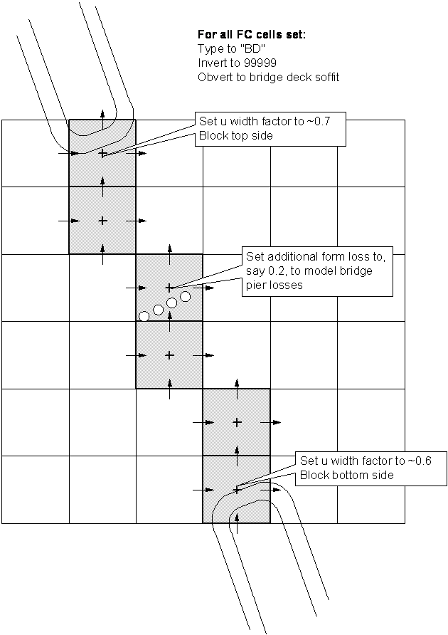
Figure 7.40: Setting FC Parameters for a Bridge Structure
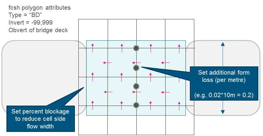
Figure 7.41: Setting FCSH Parameters for a Bridge Structure
7.4.7 Unsupported Features in TUFLOW Classic
The following features are not supported in TUFLOW Classic. TUFLOW HPC is required to access these features:
- Parallelisation / utilising GPU Hardware (Section 1.1.5.3)
- Wu turbulence approach (Section 7.3.2.4)
- Topography Sub-grid Sampling (Section 7.3.3)
- Quadtree grid refinement (Section 7.3.1)
- Groundwater with multiple sub-surface layers and horizontal hydraulic conductivity (Section 7.3.5.2)
- Non-Newtonian Flow (Section 7.3.6)
