10.2 1D and 2D Domain Linking Theory
TUFLOW 1D and 2D domains can be linked in a variety of ways. Common configurations, as shown in Figure 10.1, include:
- 1D culverts through 2D embankments.
- 1D pipe networks underneath the 2D domain.
- Nesting of a 1D open channel (e.g. creek or river) through a 2D domain.
- Connection of a broader 1D network catchment model to a high resolution 2D domain.

Figure 10.1: 1D/2D Linking Configurations
There are two types of 1D/2D linking options available:
- Head (water level) boundaries to the 2D cells (HX); and
- Source boundaries to the 2D cells (SX).
These are described in the sections below.
10.2.1 HX 2D Head Boundary
The HX terminology is derived from a Head boundary being applied to the 2D cell using data from an eXternal 1D scheme. This type of connection can be used to connect TUFLOW 2D with the 1D schemes of ESTRY (TUFLOW 1D), SWMM, Flood Modeller and XPSWMM. HX lines are typically used along riverbanks to define the 1D-2D exchange when 1D is used for in-channel representation, linked to the floodplain in 2D (commonly referred to as, 1D nested open channel modelling).
For 1D nested open channel modelling, the HX cells are defined using HX lines, connected to 1D nodes (i.e. the start and end of 1D channel lines) via connection (CN) lines. HX and CN line type objects are defined in the 2d_bc format layer. The 2d_bc layer is often renamed with the prefix 2d_hx should the modeller choose to store the HX lines in their own layer(s). The CN lines are snapped to the 1D nodes and vertices along the HX line.
The open channel area modelled by 1D must be deactivated from the 2D domain (2d_code: code = 0) otherwise the flow down the open channel will be duplicated in both the 1D and 2D domains. These model features are presented in Figure 10.2.
When TUFLOW carries out the hydraulic calculations, water level information at the 1D nodes is transferred to the HX line vertices that are connected to the 1D nodes via the CN lines. Along the HX lines, between the connected vertices, the water levels are linearly interpolated.
A HX line must have a CN line connected to each of its ends, along with any connections from intermediate 1D nodes to HX line vertices. Not every HX vertex has to have a 1D node connected. However, should a 1D node not be connected, the water level from that 1D node will not contribute to setting the water level profile along the HX line and undesirable results may occur.
If a single 1D node is connected to both ends of a HX line, the water levels in the 2D cells along the HX line will all be the same thereby producing a horizontal water level profile along the HX line. This approach is typically used for upstream boundaries into a 2D domain, and the line must be roughly digitised perpendicular to the flow (alternatively use a 2D QT boundary which automates this set up).
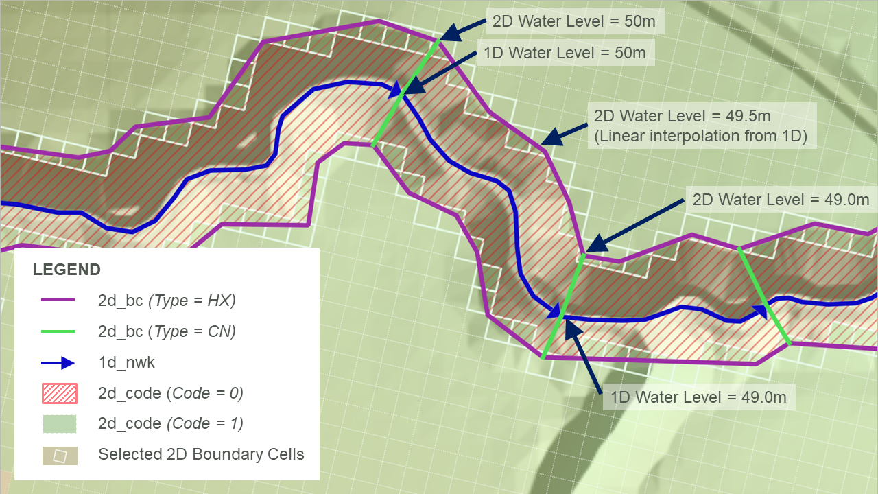
Figure 10.2: HX Connection: Nested 1D Open Channel – Plan View
Flow can either enter or leave HX cells. The volume of water entering or leaving the cells is added or subtracted from the connected 1D nodes to conserve mass. The HX link preserves momentum in the sense that the velocity field is assumed to be undisturbed across the link, however, the solution across the HX line is not a complete 2D solution as the velocity field on the inactive side of the HX line is assumed, not calculated. The 2D velocity direction is not influenced by the direction of the linked 1D channel.
Because of the momentum preservation, the HX link approach produces a superior 1D-2D linking performance where complex flow behaviour occurs (e.g. river/floodplain interactions) than using a flow source approach such as applying a weir flow equation across the link. Figure 10.3 shows an example of the preservation of momentum across HX lines (shown in light purple) as water flows across a meander where the main channel is represented in 1D.
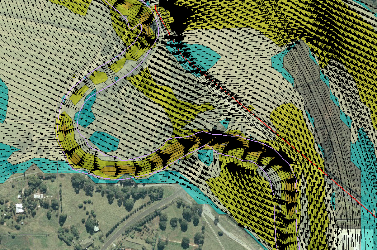
Figure 10.3: HX Connection: Example of Momentum Preservation across HX Lines
The elevations of 1D-2D boundary cells determine when water can transfer between the 1D and 2D. Water level is calculated at the cell centres in the 2D engine (see Section 7.1.3), once the water level in the 1D node exceeds the elevation in the HX cell, water can enter or leave the cell. As such, an accurate definition of the 2D HX cell centre elevations is important. If a levee aligns with the HX line, a 2d_zsh thick breakline is recommended along the levee to ensure that the 1D-2D boundary cell elevations are consistent with the levee or spill crest.
In the four panels of Figure 10.4, the 2D HX connection is shown in section view at four differing water level stages:
- Panel 1: In bank flow: the water level in the 1D section is below the 2D cell elevation and no flow is occurring across the 1D-2D connection.
- Panel 2: Spill into the floodplain: the water level in the 1D section is above the 2D cell elevation along the left bank (but not the right bank). In this case, water is spilling from the 1D channel into the 2D floodplain on the left bank.
- Panel 3: Flow from floodplain: the water level in the 1D is below the water levels on the 2D floodplains and water will drain from the 2D domain into the 1D channel, which typical occurs during a flood recession.
- Panel 4: Perched floodplain: the flow is still moving from the 2D into the 1D on the left bank, however, on the right bank, the water level in the floodplain is below the 2D HX cell elevation and no flow is occurring (the water is perched).
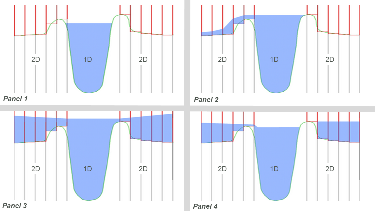
Figure 10.4: HX Connection: Nested 1D Open Channel – Section View
In addition to 1D-2D connections associated with nested 1D open channel / 2D floodplain situations, HX connections are also used to connect a 2D domain embedded within a broader 1D network representing the upstream and/or downstream river sections further afield. In Figure 10.5, HX lines are shown along the upstream inflow to the 2D Domain as purple lines, the CN lines are shown in green. The CN lines are snapped to the 1D node at the end of the 1D network and the two vertices at either end of the HX line.
The water level at the 1D node is uniformly applied to the HX cells wherever the water level exceeds the cell ZC elevation. As the water level applied along the HX line will be horizontal the HX line must be digitised roughly perpendicular to the expected flow direction. Should the line not be perpendicular, circulatory flows maybe generated, so check that the flow patterns along HX lines appear to be reasonable.
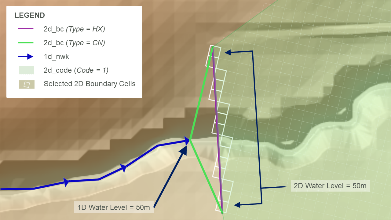
Figure 10.5: HX Connection: External 1D Network Boundary Connection
Note that for all HX links, the cell centre elevation (ZC) at a HX cell must be above the 1D bed level (interpolated between connected 1D nodes) otherwise an artificial flow across the link will be produced. To enforce this, TUFLOW produces an error message during the model initialisation, and terminates the simulation, if the interpolated 1D node elevation exceeds the 2D HX cell centre elevation (ZC). The ERROR message(s) are geo-referenced to easily identify the HX cells that lie below the 1D bed profile.
10.2.2 SX 2D Flow Boundaries
The SX terminology is derived from a Source boundary being applied to the 2D cell using data from an eXternal 1D scheme. This type of connection can be used to connect TUFLOW 2D with the 1D schemes of TUFLOW 1D (ESTRY), Flood Modeller, SWMM and XPSWMM. SX connections are typically used to transfer flow between 1D and 2D for 1D structures and at pits/drains/gully traps that capture water into the pipe network. Unique to SWMM, when using it as the 1D solver, an SX connection is only required at the downstream end of a 1D culvert (it uses a HX link at the upstream end due to limitations of the SWMM software). SX can be connected to the surface water (see Section 10.2.2.1) or to the groundwater (see Section 10.2.2.2).
At SX connections, the water level at the 1D node is reset every timestep as the average water level along the 2D SX cell(s). Conversely, the flow into or out of the 1D element feeds into the 2D SX cell(s) as a flow of water with the water level at the 2D cells computed as part of the 2D SWE solution. As the water level at the 1D node is set based on the water level in the SX cells, the storage in the 1D node is not used computationally in the 1D. Where there is an SX connection to 2D cell(s) from a 1D node, the average 1D node storage is distributed across the connected 2D SX cells.
SX objects are digitised in the 2d_bc layer and have the type set to “SX”. They can either be a point (a single SX cell), line (multiple SX cells) or region object (multiple SX cells). When using the SX line and region objects, these are joined to the 1D nodes with a single CN type object, also in the 2d_bc layer, as shown in Figure 10.6. The (2d_bc) SX point, line and region objects are shown in purple, the (2d_bc) CN lines are shown in green, and the cells selected for the SX 1D-2D connection are highlighted in white.
- When using an SX point, the point object needs to snap to the 1d network (1d_nwk) at the nodes (end of the culvert). A single 2D cell is selected for the 1D-2D SX connection.
- When using an SX line, a connection line snaps to the SX line and the 1d network (1d_nwk) node. Multiple 2D cells are selected for the 1D-2D SX connection. If the line does not select any 2D cells a single 2D cell is selected based on the line’s mid-point.
- When using an SX region, a connection line snaps to a vertex of the SX region and 1d network (1d_nwk) node. Multiple 2D cells are selected for the 1D-2D SX connection based on whether the 2D cell centre falls within the region. If the region does not select any 2D cells a single 2D cell is selected based on the region’s centroid.
10.2.2.1 SX 2D Flow Boundary to Surface Water
The flow onto the SX cells is treated as a source flow, i.e. it can be positive or negative in magnitude but has no directional component. If there is more than one SX cell connected, the flow is, by default, proportioned via the depths in the 2D SX cells. The SX Flow Distribution Cutoff Depth command can be used to control the depth of water below which an SX cell does not receive flows from the connected 1D element.
Note that when connecting an SX connection for a 1D structure it is important to ensure that the width of connected SX cells at the structure invert (and higher levels for irregular shaped structures) is equal or more than the width of the 1D structure. This check should take into account whether any of the 2D SX cells are dry at the level being checked. If the width of water flow across the SX cells is less than the flow width of the 1D structure, the 2D SX cells become the constriction and instabilities or unrealistic flow patterns may result.
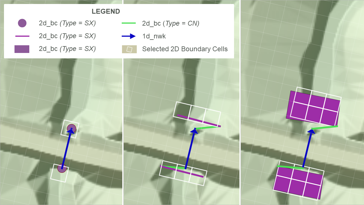
Figure 10.6: SX Connection Options
The lowest 2D SX cell (based on the ZC, cell centre, elevation) must be below the 1D bed level (invert) otherwise mass can be artificially generated. TUFLOW produces an ERROR message during the model initialisation and a simulation will not run if a 1D node elevation falls below the lowest 2D ZC SX cell elevation.
In addition to culverts through embankments, SX connections are used to connect 1D pipe network inlets (pits) to the ground surface, which is modelled in 2D. An example is presented in Figure 10.7 and Figure 10.8. The SX connections are used to transfer flow between the 1D pit/pipe network and the 2D domain. To make the workflow more efficient, pit SX connections can be simply defined using one the pit attributes in a 1d_nwk or 1d_pit layer, thereby removing the need to have a 2d_bc layer - see Section 5.10.2.
A model using the SX to surface water functionality is provided in the 1D Structures Example Model Dataset on the TUFLOW Wiki.
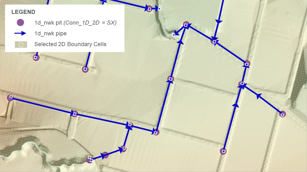
Figure 10.7: SX Connection: Pipe Network – Plan View
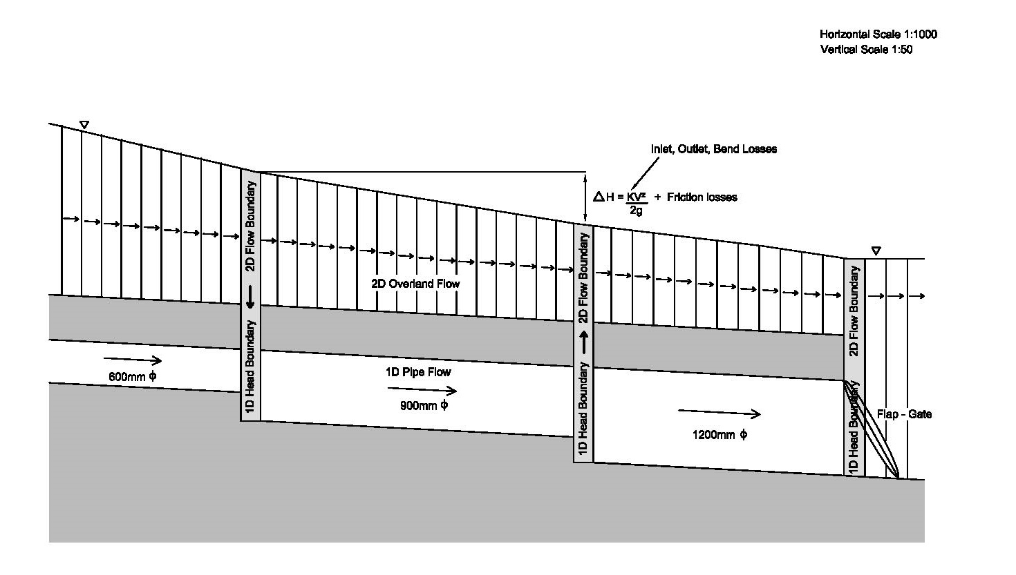
Figure 10.8: SX Connection: Pipe Network -Section View
10.2.2.2 SX 2D Flow Boundary to Groundwater
Groundwater connections to 1D elements are useful for representing modelling situations where water infiltrates into or is extracted from the soil other than the default connection to the 2D surface water. These situations can arise in green infrastructure systems, which may incorporate intentionally infiltrating water into the groundwater, draining water from the groundwater or both. For example, retention basins designed to enhance infiltration through natural or artificial soils and to slowly drain stored groundwater to reduce water levels ahead of future rainfall events. Water seepage into the groundwater can be modelled in 1D or 2D, but drains are modelled in 1D.
To define a groundwater connected in a 1D network, a “SX” boundary is used in the 2d_bc GIS layer, with the “GW[1 - 9]” flag specifying the connection to a groundwater layer (see Table 8.6). The connected groundwater layer number follows the “GW” flag. For example, “GW2” would be the flag for a connection with groundwater layer 2. The direction of flow and discharge are determined using the same principles as a SX connection to surface water (see Section 10.2.2.1), except that the 2D water level is replaced by the groundwater pressure level. As such, the 1D node is assigned a water level equivalent to the groundwater pressure level.
In most cases, groundwater to SX connections have some connection mechanism that must be represented in the model to control how much flow is transferred. For example, the flow through slotted or perforated pipes commonly used in detention basins to drain water from the soil can often be approximated using the orifice equation (Equation (5.22)) but manufacturers may have other defined relationships for how much water is extracted for a given pressure level.
The depth vs discharge relationship used to define these flows is based on the pressure head in the groundwater layer and the connection attributes (slotted pipe width or size and number of holes in perforated pipe and pipe lengths). The same relationship is used for ESTRY and SWMM but applied differently due to connectivity requirements for the engines:
- ESTRY: A separate inlet or pit is not required. Instead, a “Q” or “M” channel is typically used with the groundwater pressure level vs discharge relationship to represent the interchange between groundwater and 1D. See Section 10.3.5.
- SWMM: An inlet is required at the 1D node (either a junction or a storage node). This inlet is typically a generic inlet (see Table L.17) using a groundwater pressure level vs discharge relationship. See Section 10.4.3.
Guidance for generating depth vs discharge curves is provided on the TUFLOW Wiki Groundwater Modelling Advice page.
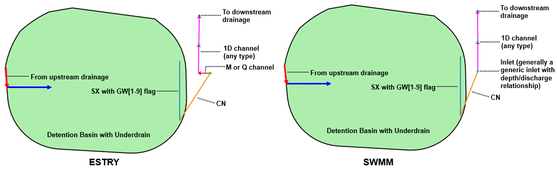
Figure 10.9: SX 2D Flow Boundary to Groundwater: ESTRY and SWMM