3.2 Model Resolution (Discretisation)

3.2.1 1D Networks

The veracity of a 1D model domain is primarily dependent on the resolution with which on ground conditions are represented. The nature of this representation is typically a result of a balance between required resolution and the commensurate manual setup effort, the latter of which can be significant. Some approaches that can be used in establishing this balance include:

• Carefully determining where and to what extent 1D networks are required in order to address study goals, and
• Combining multiple 1D channels or structures into single model elements where appropriate

3.2.2 2D Cell Sizes

The 2D cell size defines the resolution of the 2D hydraulic calculations. As for 1D simulation, this cell size needs to be sufficiently small so as to reproduce required hydraulic behaviours, but not so small that simulation times are impractical. In order to assist with this cell size selection, Table 3.1 lists general recommendations for minimum cell count (size) relative to primary flow path widths (e.g. creeks or streets), for different TUFLOW solvers.

Table 3.1: Recommended 2D Cell Size

Solver	Minimum recommended number of cells across flow paths	Sensitivity of results to flow path orientation
TUFLOW Classic	4-6	Low
TUFLOW HPC without SGS	6-8	Medium
TUFLOW HPC with SGS	3-4	Very Low (assumes terrain data is a finer resolution by a factor of 2 or more)

Resolution may vary from these recommendations if:

1. 1D is used for primary flow path definition and 2D only for floodplains: 2D cell size can increase.
2. Using HPC’s SGS feature (refer Sections 3.2.3 and 7.3.3): 2D cell size can increase.
3. Using HPC’s Quadtree feature: 2D cell size can increase outside areas of interest.
   
4. Small cells are contained within deep water flow paths. These settings will slow down models considerably and should be avoided through use of SGS.

More broadly, cell size result convergence sensitivity testing (see Section 3.2.4) is the most robust way to verify 2D cell size selection. It should be completed early in the model development process.

3.2.3 Sub-Grid Sampling (SGS)

Without SGS, TUFLOW samples an underlying DTM only at cell centres and faces when assigning bathymetry to a computational grid. Cells and faces are then effectively flat-bottomed storage boxes and conveyance channels, respectively. This approach discards any higher spatial resolution DTM data that may have been available. As an example, Figure 3.4 presents a 20m hydraulic model grid, overlaying a 1m DTM. In this case only 2 to 3 grid cells span the river channel, and fewer in some of the floodplain channels and road embankments. As such, the sub-grid (sub-cell) scale topography available in the DTM is underutilised and a poor representation of bathymetry is likely. Traditional solutions to this problem would typically have involved specifying smaller cell sizes, at considerable computational penalty.

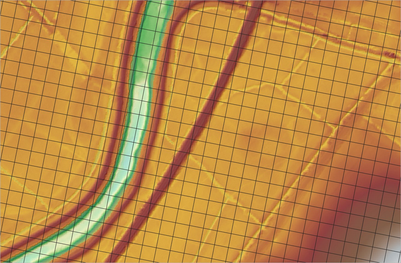
Figure 3.4: 20m grid size shown against the 1m DTM

Rather than using a single elevation value for the grid cell storage calculations, Sub-Grid Sampling (SGS) topography sampling extracts sub-grid data from an underlying DTM to develop a non-linear relationship between water surface elevation and cell volume (i.e. storage capacity). SGS also generates a non-linear relationship between water surface elevation and cell face area and width (i.e. wetted perimeter) to improve the representation of fluxes and conveyance across cell faces. As such, whilst the SGS approach still computes a single water level for each cell, higher resolution terrain data than the grid cell size is utilised within the 2D hydraulic modelling, which improves simulated results. The conceptual difference between traditional and SGS topography sampling approaches is presented in Figure 3.5.

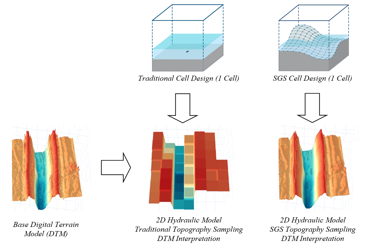
Figure 3.5: 2D Topography Sampling Concept and DEM Interpretation (Traditional vs SGS)

SGS is a feature of TUFLOW HPC - it is not available in TUFLOW Classic. If using TUFLOW HPC, SGS is recommended when the available DTM data is finer than the model resolution. SGS is discussed further in Section 7.3.3.

3.2.3.1 Benefits of SGS

Benchmarking has shown the benefits to be substantial for at least the following situations:

• Catchment scale models flow much more effectively with water not being “trapped” by a coarse cell resolution, and, importantly, excellent cell size convergence (i.e. demonstrating that by reducing the cell size(s) the model results do not demonstrably change) at much coarser cell sizes. Figure 3.6 shows the flow hydrographs for a Quadtree direct rainfall whole of catchment model using two base cell size resolutions. The Hi-Res Quadtree grid has a base cell size half that of the Lo-Res grid. The grey and yellow hydrographs show results from models without SGS enabled and their marked difference in peak flow, shape and timing demonstrate significantly different results between the two resolutions, and a cell size convergence test failure and the need for further refinement of the cell sizes (and much longer run times). In contrast, the blue and orange hydrographs are from the same model, however with SGS turned on and show very similar results between the two resolutions, thereby demonstrating excellent cell size convergence and the ability to use the faster running Lo-Res model for day-to-day modelling.

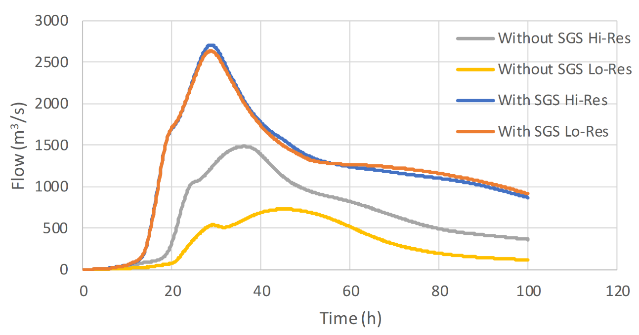
Figure 3.6: Model Convergence with and without SGS

• The sensitivity of results to mesh size is greatly reduced and the sensitivity to mesh orientation is almost eliminated. With SGS a 2D regular mesh model can be rotated or have a change in cell size without impacting the accuracy of the results compared with much greater and sometimes unacceptable changes in results for the traditional elevation per cell approach (Kitts et al., 2020).
• Disturbed flow fields that can be apparent along a “saw-tooth” regular grid wet-dry boundary completely disappear, with no spurious additional head losses generated and the results consistent with a well-designed flexible mesh. This has major benefits in that open channels can now be accurately modelled using TUFLOW HPC using coarse cell sizes at any orientation to the channel, removing the need to utilise 1D open channels carved through the 2D domain. The images and charts below show benchmarking to a U-Bend flume test for without SGS and with SGS. SGS causes a much smoother flow field to occur and importantly the head drop around the bend is correctly modelled with SGS on. The red highlighted cells indicate those cells that are partially wet with SGS on. The charts show the longitudinal profile on the outside (orange), centre (blue) and inside (grey) of the bend with lines being modelled and points measured – as shown, with SGS off the upstream water level is over predicted as shown by the red circle.

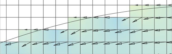
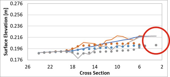
Figure 3.7: Longitudinal Profile without SGS

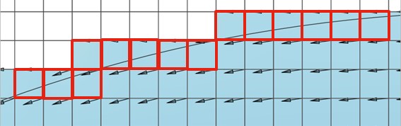
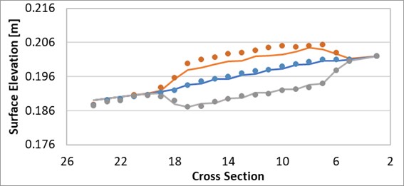
Figure 3.8: Longitudinal Profile with SGS

In summary, utilising SGS means:

• The storage and conveyance of the model is more accurately represented.
• Cell Size Result Convergence, discussed in the following section, can typically be achieved using a larger cell size when using SGS, compared to when not using SGS.
• Faster simulation times.

3.2.4 Cell Size Results Convergence

Solution convergence to cell size refers to the tendency for model simulation results to trend towards a common answer as cell size decreases. This behaviour occurs due to the discretisation of topographic features at a finer and finer resolution and should trend towards a closer and closer reproduction of reality. Conversely, by using too coarse a cell size, the results can become affected by the inaccuracies introduced by trying to emulate reality with a poor (i.e. coarse) representation of the topography.

The practical test required to complete cell size convergence involves progressively reducing a model’s cell resolution and comparing the results. The process aims to identify the largest cell size possible to achieve a consistent simulation result (i.e. a simulation result that does not introduce inaccuracies caused by using an excessively large cell size). Identifying this optimum cell size will avoid the situation where an unnecessarily small cell size is chosen, which subsequently translates to longer than necessary simulation times with no significant improvement in simulation result. Figure 3.9 demonstrates this concept. The 40m cell resolution model produces a result at the reporting location that is consistent with the finer cell sizes, whereas for larger cell sizes (60m and higher) the results are not consistent demonstrating they are too coarse to accurately reproduce the hydraulics. As the 40m resolution simulation time is significantly less than smaller cell sizes, it represents the optimum cell size value to achieve reliable results in the shortest run time.

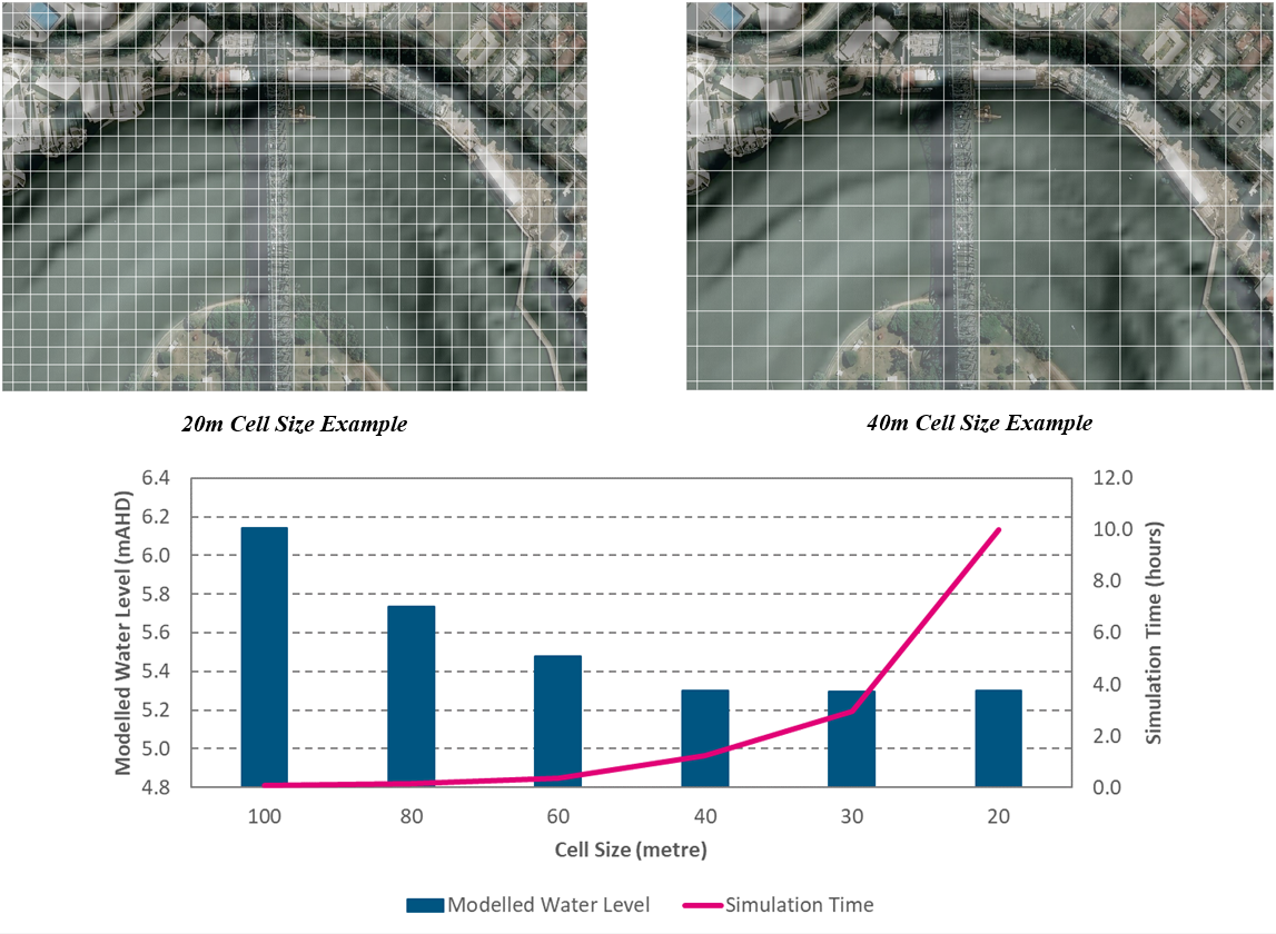
Figure 3.9: Cell Size Convergence Concept Example

The decision as to whether or not the model results are “converged” is subjective and will depend on the purpose of the modelling and specifically what the “essential results” are. For some studies they may be water surface elevation in a region of interest (e.g. a town), and for another study the essential result may be the peak flow at a particular location. The exact approach taken to establish cell size convergence is up to the user, but we present a selection of methods below that may be useful. Whether one of the following methods are used, or another method, it is important to document all testing and if necessary engage stakeholders in the decision-making making process.

• Comparing flood extent. This simple approach may be performed by overlaying 2D maps of flood extent from sets of results calculated at different cell sizes. The user might start with a relatively large cell size and then keep halving the cell size until the results become acceptably similar. The 2^nd to last (i.e. penultimate) cell size is then the one that may be considered as sufficiently converged.
• Comparing flow response. Another approach, well suited to highly transient models, is to place flow lines across a primary path at important locations, and plot the flow as a function of time for the different sets of results. Again the user may start with a large cell size and refine until the results become acceptably similar.
  
• Creating a result vs cell size plot. This method is more useful when there is a specific result of interest (e.g. the peak water level at a particular location such as used in the example above). With this method the result of interest is plotted as a function of cell size. This method allows the user to estimate the error between the model result (at a given cell size) and their estimate for the “perfectly converged” result. The largest cell size for which the error is within some defined tolerance may then be considered sufficiently converged. If the resulting plot is “noisy”, then this can indicate a possible error with the modelling setup (e.g. an embankment not being resolved at larger cell sizes, or possibly a model instability). Note, this approach may hide poor convergence elsewhere and is rarely used unless multiple sites are compared and convergence sought for all of them.
• Histogram of variation. This approach involves comparing large lists of results (e.g. water levels at say 100 or more locations) and generating a histogram of differences between the results at the test cell size and the results at the finest feasible cell size. The user may then define, for example, a criterion such that 95% of the results must be within +/- <some tolerance> of the results from the finest feasible cell size. The user determines the largest cell size that satisfies the criterion, and deems that as sufficiently converged.

SGS (see Section 3.2.3) has a significant beneficial impact on cell size convergence. In many situations, a model using SGS may meet the required convergence criteria with a cell size that is much larger than when SGS is not used (Huxley et al., 2022).

Finally, the cell size convergence testing maybe affected by the viscosity formulation (Section 7.1.4). In particular, the Smagorinsky viscosity formulation can cause results to be more sensitive to cell size, and can allow the model results to diverge with decreasing cell size once the cell face width becomes less than the depth. The Wu viscosity formation (default for TUFLOW HPC) has proven to be superior to Smagorinsky in terms of reduced sensitivity to cell size and convergence of results.