10.3 TUFLOW 1D (ESTRY) to TUFLOW 2D Linking
Linked TUFLOW 1D and 2D domain models use 2D HX and 2D SX boundary types connected to 1D nodes (1d_nwk layer) using CN lines or points in the 2d_bc layer, as described in Section 8.4. The recommended approach for HX and SX connections are summarised in the following sections.
10.3.1 1D Open Channel and 2D Domain Linking
2D_bc HX boundaries are preferred for transitioning between 1D domains and 2D domains (shown in Figure 10.5) or when nesting a 1D open channel network within a 2D domain (shown in Figure 10.2).
An example of these HX connections is provided in TUFLOW Tutorial Module 11. The TUFLOW Wiki 1D2D Boundary Configuration Guidance also includes useful guidance on how to stabilise problematic 1D/2D TUFLOW HPC HX connections.
10.3.2 1D Structures Embedded within 2D Domains
2D_bc SX boundaries are preferred for inserting 1D culverts inside a 2D domain. For example, a 1D culvert underneath a road embankment, as shown in Figure 10.6.
An example of these SX connections is provided in TUFLOW Tutorial Module 3. The TUFLOW Wiki 1D2D Boundary Configuration Guidance also includes useful guidance how to stabilise problematic 1D/2D SX connections.
10.3.3 1D Pipe Network Pits linked to 2D Domains
Pits/Inlets within an urban drainage environment provide bi-directional connectivity between the urban surface represented by 2D domains and the 1D sub-surface pipe network. They use the SX type linking described in Section 10.2.2.1. To simplify the model setup process the SX connections are automatically created by setting the Conn_1D_2D attribute for the pit/inlet point object to “SX” in the 1d_pit or 1d_nwk layer. The type of pit is defined using the ‘Type’ attribute:
- “C” pits use zero length circular culverts to calculate the flow transferred between the 1D network and 2D domain.
- “R” pits use zero length box culverts to calculate the flow transferred between the 1D network and 2D domain.
- “W” pits use the weir equation to calculate the flow transferred between the 1D network and 2D domain.
- “Q” pits use a user-specified Depth-Discharge curve to transfer flow between the 2D domain and the 1D domain, based on the 2D water depth.
Section 5.10.2 contains information about the specification of pit parameters. A pipe network model example is provided in TUFLOW Tutorial Module 5.
10.3.4 Virtual Pits linked to 2D Domains
Compared to the above-mentioned approach, virtual pits are an alternative way to model pits/inlets where the sub-surface pipe network is not being modelled. The flow entering a virtual pit can either be discharged back into the model further downstream or permanently extracted from the model. There are three main approaches to using virtual pits:
- Virtual Pit Inlets (Type ‘VPI’) only are used to extract flow from the model. One examples would be where there is no or insufficient data on the pipe network. Another example is where the pipe network flow discharges to a river (assuming the level in the river does not affect the flow into the pits) and no pit surcharging back onto the 2D domain occurs.
- VPIs are used in with Virtual Pipe Outlets (VPOs), which allow the flow into VPIs to be discharged back onto the model. VPIs can be allocated to specific VPOs via a common network ID. VPOs can have a limiting outlet flow. Once the VPO flow reaches the limit, the excess flow is surcharged back through VPIs, which can be prioritised as to which ones surcharge first. By default, the routing of flow between VPIs and VPOs on the same network is instantaneous (i.e. no lag). However from the 2023-03-AB build, it is possible to apply a lag or shift to the flows from the inlet to the outlet by using the 1d_pit Lag_Approach and Lag_Value attributes.
- Flows from VPIs can be connected to 1D channel nodes to drain flow from the 2D surface and reintroduce them to the 1D domain further downstream. This is a useful approach to modelling the major sub-surface drainage system as a pipe network and the minor system as VPIs feeding into the major system.
Section 5.11 contains more information about virtual pits. Models using these model configurations are provided in the 1D Pipe Network / 2D Floodplain Modelling Example Model Dataset on the TUFLOW Wiki.
As previously mentioned, pits, virtual pits and nodes can be automatically connected to 2D domains using the 1d_nwk Conn_1D_2D attribute (see Table 5.26 and Table 5.25). If Conn_1D_2D is set to “SX”, TUFLOW automatically connects the upstream end of the pit channel or node to the 2D domain.
- For this automated 1D-2D SX connection to establish, it is a requirement that the 2D cell must be active (2d_code, Code = 1). If no active 2D cells are found from any 2D domain, a WARNING 2122 or 2123 is issued.
- The command Pit Default 2D Connection can be used to set the global default value for the 1d_nwk Conn_1D_2D attribute.
- By default, TUFLOW will connect the 1D pit/virtual pit/node to one or more 2D cells at pit connections. The number of 2D cells selected is a function of the flow width of the pit inlet (including the effects of the Number_of and Width_or_Dia 1d_nwk attributes), or the total flow width of the channels connected to the node. The total width of the 2D cells selected is always more than the pit inlet width or width of channels. For example, a width of 3.6 m on a 2 m grid selects two cells. The advantage of selecting more than one 2D cell is to provide enhanced stability at the 1D/2D connection when the 1D flow width exceeds the 2D cell size. The number of 2D connection cells is limited to 10 per pit inlet.
- The 1d_nwk Conn_No attribute can be used to change the number of 2D cells connected as follows:
- A positive value adds that number of 2D cells to the automatic number. In the example above, if Conn_No is set to 1, three (2 + 1) 2D cells are connected. The upper limit is 10 connected cells.
- If Conn_No is negative, this ignores the automatic approach and fixes the number of 2D cells connected to the absolute value of Conn_No. For example, a value of -1 would only connect the pit or node to one (1) 2D cell irrespective of the width.
- A positive value adds that number of 2D cells to the automatic number. In the example above, if Conn_No is set to 1, three (2 + 1) 2D cells are connected. The upper limit is 10 connected cells.
- If more than one 2D cell is being connected, there are two approaches available for how the 2D cells are selected.
- For pits, the default is the G (on Grade) option that selects the 2nd, 3rd, etc… cells by traversing to the next highest 2D cell that neighbours the 2D cell(s) already selected (this includes diagonal cells, i.e. all 8 cells around a cell are considered). These cells are also automatically lowered to the same height as the first cell so that their ZC value is at or below the pit inlet.
- For nodes, the default is the S (Sag) option that selects the 2nd, 3rd, etc… cells by traversing to the next lowest 2D cell. The ZC values of these cells are not changed as they are already at or below the node invert.
- For pits, the default is the G (on Grade) option that selects the 2nd, 3rd, etc… cells by traversing to the next highest 2D cell that neighbours the 2D cell(s) already selected (this includes diagonal cells, i.e. all 8 cells around a cell are considered). These cells are also automatically lowered to the same height as the first cell so that their ZC value is at or below the pit inlet.
- The above approaches can be changed using the G (Grade) and S (Sag) flags for the 1d_nwk Conn_1D_2D attribute. The G approach is that adopted by default for pits and S for nodes. To override the default approach, specify G or S as appropriate. For example, if the S approach is preferred for a pit that is draining a depression, specify an S flag for the Conn_1D_2D attribute (i.e. “SXS”). Note SX must come first before an optional flag is specified.
Note, the conventional 1D-2D link approach using 2d_bc SX points, lines or regions can still be used to connect 1D channel ends. This gives the user complete control over the 2D cells selected and may still be preferred in situations where large 1D structures are being connected to 2D cells.
10.3.5 TUFLOW 1D (ESTRY) linked to Groundwater
ESTRY can connect directly with groundwater using SX connections as described in Section 10.2.2.2 (see Table 8.6). Groundwater connections to 1D (ESTRY) often include perforated or slotted pipes to convey flow to or from the 1D network. These are typically modelled using a depth vs discharge relationship implemented in ESTRY as a “M” channel (see Section 5.8.1) or a “Q” channel (see Section 5.8.2) directly downstream of the connecting node, as shown in Figure 10.10. The depth vs discharge relationship is often based on the orifice equation (Equation (5.22)) where the coefficient will vary depending on the design of the groundwater to 1D connection.
Guidance for generating depth vs discharge curves is provided on the TUFLOW Wiki Groundwater Modelling Advice page.
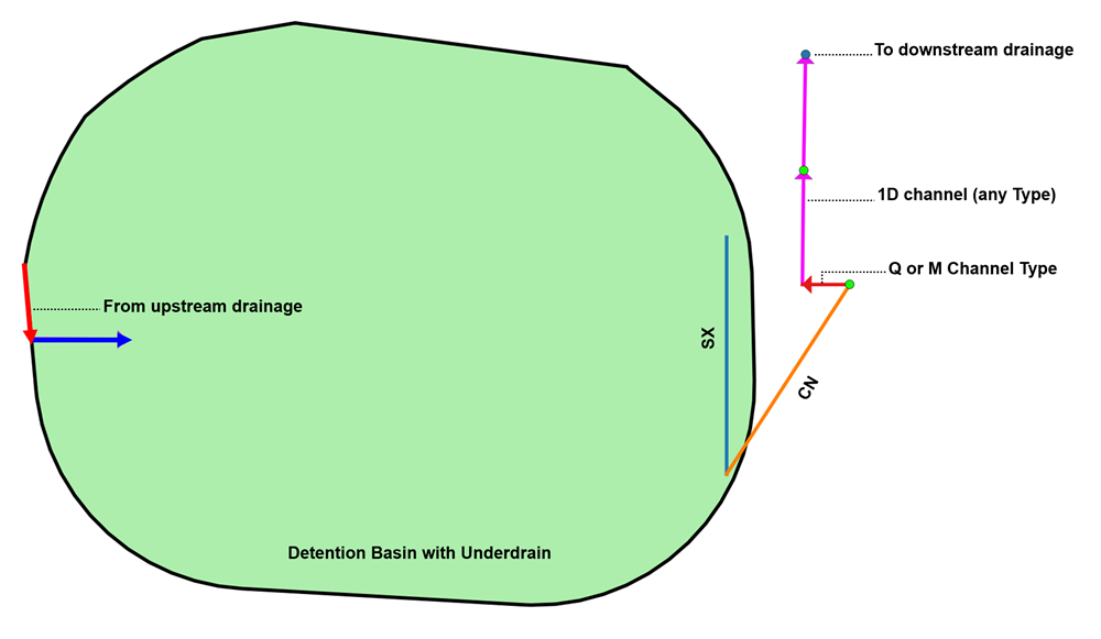
Figure 10.10: Groundwater Linking to 1D - ESTRY