11.3 Time-Series Outputs
Time-series results (sometimes referred to as Plot Output) produces output for graphing in charts and profiles. The data output are specified using the Map Output Data Types command, at an interval specified by the Time Series Output Interval command.
Time-Series data can be output for 1D domains (Section 11.3.1) and 2D domains (Section 11.3.2). If the total flow across the floodplain is required for a 1D/2D model where the river is in 1D and the floodplain in 2D, flows can be combined using Reporting Locations (Section 11.3.3). The Structure Reporting feature outputs time-series and summary data for structures (Section 11.3.4).
There are two formats available for time-series outputs: comma-separated values (.csv) (the default) and NetCDF (.nc). One of the advantages of NetCDF is all the timeseries output is in a single compressed .nc file, rather than multiple uncompressed .csv files. To change the format use Time Series Output Format command.
It is possible to write 1D and 2D time-series outputs as the simulation progresses, using the Write PO Online command.
11.3.1 1D Time-Series Output
Time-series data output from 1D domains is available for a range of hydraulic parameters. The Output Data Types ECF command or the 1D Output Data Types TCF command controls the types to output. The options are:
- A: flow area at channels (m2 or ft2);
- E: energy at nodes (m or ft);
- H: water level at nodes (m or ft);
- Q: flow at channels (m3/s or ft3/s);
- QI: integral flow at channels (m3 or ft3);
- S: structure and grouped structure output (see Section 11.3.4);
- V: velocity at channels (m/s or ft/s); and
- Vol: volume at nodes (m3 or ft3).
Note: Metric (SI) units are TUFLOW’s default. To use imperial units, ensure
To review the 1D time-series data see 15.2.
11.3.2 2D Time-Series Output
Time-series data output from 2D domains is available for a range of hydraulic parameters (as listed in Table 11.9). Output takes the form of time-series hydrographs (referred to as PO – Plot Output) or longitudinal profiles (LP) over time.
This is carried out by creating one or more GIS layers containing points, lines and regions that define the locations of PO and LP output. Figure 11.4 illustrates how 2d_po objects are interpreted.
The start time for PO and LP output and the output interval is set using Start Time Series Output and Time Series Output Interval. If no start time is specified the simulation start time is used. If no output interval is specified the simulation will stop with ERROR 0046 to prevent excessive amounts of memory and disk space from being used.
The output is written to a .csv file and also to the _TS layer (refer to Section 15.2.4). 2D domain time-series (PO) output is synchronised with 1D domain output by default. This allows both 1D and 2D time-series to be placed in the _TS layer. Set Output Times Same as 2D to OFF in the .ecf file if 1D and 2D time-series data is not to be synchronised. In this case, no 2D PO is written to the _TS layer.
Maximums and minimums are output to four additional rows near the top of the _PO.csv file, and columns in the _LP.csv files, containing the Maximum, Time of Maximum, Minimum, and Time of Minimum values. The _TS GIS layer also contains the tracked values. For TUFLOW Classic this information is tracked every computational timestep. For TUFLOW HPC the maximum/minimum values are post-processed at the end of the simulation based on the Time Series Output Interval, not every computational timestep. Tracking of maximums and minimums can be disabled by setting the Maximums and Minimums Time Series command to OFF in the .tcf file.
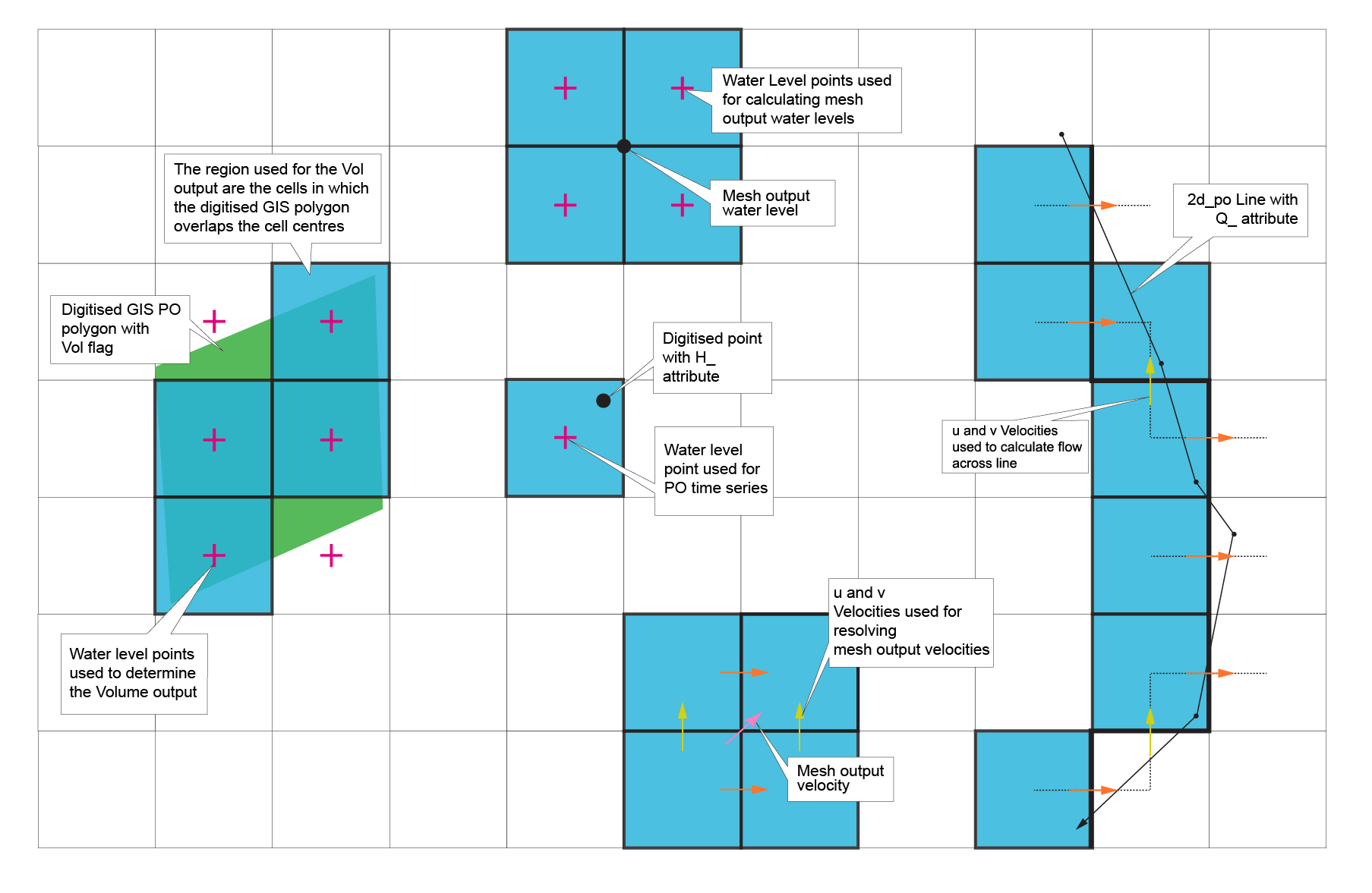
Figure 11.4: Interpretation of PO Objects and Map Output
11.3.2.1 Plot Output
The data types available for PO are as listed in Table 11.9, noting that only supported object types (i.e. Point, Line and Region) for the data type are documented in the table. PO data is read into a simulation using the Read GIS PO .tcf command. This is carried out by creating one or more GIS layers containing points, lines and regions that define the locations of PO and LP output. Figure 11.4 illustrates how 2d_po objects are interpreted.
| Flag | Description | Comments |
|---|---|---|
| CI | Cumulative Infiltration |
Point: Represents the current water content of each layer. This value may increase or decrease depending on the flows into and out of the cell (it is not the cumulative value). Units are mm or in (if using |
| D_ | Depth |
Point: Depth of the nearest cell. Line: The average depth of all wet cells along the line. Note: In TUFLOW Classic if a line with more than 2 vertices (i.e. a polyline) is used, the average water level along each line segment is output, and use of polylines is not recommended for this output type at present. TUFLOW HPC, will take the average depth along the entire polyline. Units are m or ft (if using |
| G_ | Gauge Level |
Point: Water level at the cell center of the nearest cell. If the cell is dry, the ground level (ZC) is output. Used for Read GIS Objects to record gauge levels when a receptor is first inundated. Refer to Section 11.3.3. Units are m or ft (if using |
| GWd | Groundwater Depth |
Point: Depth of water within sub-surface layer(s) (cumulative infiltration divided by porosity). Units are m or ft (if using |
| GWh | Groundwater Level |
Point: Elevation of groundwater surface (water table) within sub-surface layer(s). Units are m or ft (if using |
| GWm | Groundwater Moisture | Point: A dimensionless number in range 0 - 1 representing “fraction full” of the sub-surface layer(s). |
| GWq | Groundwater Unit Flow |
Point: Unit flow magnitude within the sub-surface layer(s). Line: Total flow passing through the given line within each sub-surface layer(s). The positive flow convention is left to right looking downstream (same as the Q_ type). Units are m2/s or ft2/s (if using |
| Gwqa | Groundwater Unit Flow Angle | Point: Angle of unit flow vector within each layer. Reported in degrees clockwise from north (i.e. a compass bearing). |
| Gwqu |
Groundwater Unit Flow U-Component |
Point: Unit flow u-component within each sub-surface layer(s). Units are m/s or ft/s (if using |
| GWqv |
Groundwater Unit Flow V-Component |
Point: Unit flow v-component within each sub-surface layer(s). Units are m/s or ft/s (if using |
| GWVol | Groundwater Volume |
Region: Total volume of water within the polygon for each layer. Units are m3 or ft3 (if using |
| H_ | Water Level (Head) |
Point: Water level of the nearest cell. If the cell is dry, the ground level (ZC) is output. Units are m or ft (if using |
| HAvg | Average Water Level |
Region: The average water level within the region (wet cells only). Units are m or ft (if using |
| HD HU | Downstream and Upstream Structure Water Levels |
Point: To associate the HU and HD objects with the QS line, all three (QS, HU and HD) must have the same ID for the 2d_po Label attribute (see Table 11.10). Note that the water levels over time are output to a 2D PO .csv file and the summary information at the flood peak to the new _SHmx.csv file. If the point or line is completely dry, -99999 is output to the .csv files. The _SHmx.csv file is currently not produced for 2D only models. Units are m or ft (if using |
| HMax | Maximum Water Level |
Region: The maximum water level within the region. Units are m or ft (if using |
| Q_ | Flow or discharge |
Line: The flow crossing the line. The flow is determined by summing the flow across cell sides whose perpendiculars intersect the line (see Figure 11.4). The flow is positive if the water is flowing away from you when looking in a direction with the start of the PO line on your left and the end of the line on your right. If digitising a flow line across a 1D channel that is carved through the 2D domain, ensure that the line is digitised so that it crosses the 1D channel where there is a change in colour in linked 2D HX cells as shown in the 1d_to_2d_check or _TSMB1d2d layers (thematically map using the Primary Node if not using MapInfo). The 1D flow can then be added manually in a spreadsheet. However, note that Read GIS Reporting Location is now the preferred method for cumulating flows across a line for 1D/2D models. See Section 11.3.3 for discussion on Reporting Locations. Units are m3/s or ft3/s (if using |
| QA | Flow Area |
Line: The flow area is calculated using the same cell sides as for Q_. An adjustment for oblique lines is made. Units are m2 or ft2 (if using |
| QI | Integral Flow |
Line: Integrates the flow (as determined for Q_ above) over time (i.e. the area under a Q_ time-series curve) (i.e. cumulative volume). If Write PO Online is set to ON, the integral flow is not calculated until the simulation is complete. Units are m3 or ft3 (if using |
| Qin | Flow In |
Region: The flow into a region. Units are m3/s or ft3/s (if using |
| Qout | Flow Out |
Region: The flow out of a region. Units are m3/s or ft3/s (if using |
| QS | Structure Flow |
Line: Same as Q_ above, but used to set up a 2D structure output (see Section 11.3.4) that will include, in addition to the 2D flow, any flows from intersected 1D structures and the split between below and above deck flows. Note the flow output to the 2D PO .csv files is only the 2D flow, while the _SQ.csv file is the combined 1D/2D structure flow. The _SQ.csv file is not produced for 2D only models. Units are m3/s or ft3/s (if using |
| QX | Flow in X-direction. |
Line: The X component of Q_ (i.e. the sum of the flows at the u-points). Units are m3/s or ft3/s (if using |
| QY | Flow in Y-direction. |
Line: The Y component of Q_ (i.e. the sum of the flows at the v-points). Units are m3/s or ft3/s (if using |
| SS | Sink Source |
Region: Sink / source flows applied within the region (rainfall, infiltration, source area inflow and SX flows). Units are m3/s or ft3/s (if using |
| V_ | Velocity |
Point: The magnitude of the resolved vector based on the two u-points and two v-points of the cell in which the point falls. Exactly which cell is selected may be uncertain if the point falls exactly on a cell’s side. Line: Velocity as Q_/QA (i.e. the depth and width averaged velocity along the line). Prior to release 2020-10-AA it used the cell in which the line starts. Units are m/s or ft/s (if using |
| VA | Velocity Angle | Point: The angle of V_ (degrees relative to east where east is zero, north is 90, etc.). |
| Vol | Volume |
Region: Total volume within the region. Units are m3 or ft3 (if using |
| Vu or Uu | u-point velocity |
Point: The magnitude of the u-point velocity (i.e. across the right hand side of the cell). Units are m/s or ft/s (if using |
| Vv | v-point velocity |
Point: The magnitude of the v-point velocity (i.e. across the top side of the cell). Units are m/s or ft/s (if using |
| VX | Velocity in X-direction |
Point: The magnitude of the velocity in the geographic X direction. This is different from the Vu if the model is rotated. Units are m/s or ft/s (if using |
| VY | Velocity in Y-direction |
Point: The magnitude of the velocity in the geographic Y direction. This is different from the Vv if the model is rotated. Units are m/s or ft/s (if using |
Table 11.10 describes the GIS attributes of the 2d_po layer.
| No | Default GIS Attribute Name | Description | Type |
|---|---|---|---|
| 1 | Type | Any combination of the two letter flags listed in Column 1 of Table 11.9 (limit of 10 flags per entry). For example, to output velocity and flow time-series for the same line, enter “V_Q_”. | Char (20) |
| 2 | Label |
Label up to 30 characters long defining the name of the time-series. The label appears at the top of the columns of data in the _PO.csv file. Spaces are permitted, but do not use commas. Read GIS Reporting Location is the preferred method for cumulating flows in 2D1D models. See Section 11.3.3 for discussion on Reporting Locations. |
Char (30) |
| 3 | Comment | Optional field for entering comments. Not used. | Char (250) |
11.3.2.2 Long Profile Output
H_ (water level) and V_ (velocity) are the only data types available for long profile (LP) outputs. LP locations and data types are initiated for a simulation using the Read GIS LP .tcf command.
Table 11.11 describes the GIS attributes of the 2d_lp layer. The 2d_lp layer(s) contain lines defining where the profile data are to be generated. Each line is given a label to uniquely define the profile in the output. The starting vertex of the line will set the distance origin for the profile.
The advantage of having TUFLOW generate the profiles directly rather than post-processing them is the outputs will be slightly more accurate due to no post-processing interpolation rounding, plus if the profile(s) are repeatedly being plotted, the plotting process can be streamlined via python scripts that use the LP outputs.
Models using 2D longitudinal profiles (2d_lp) are provided in the Output Options Example Model Dataset on the TUFLOW Wiki.
| No | Default GIS Attribute Name | Description | Type |
|---|---|---|---|
| 1 | Type | Specify “H_” to output water level. Specify “V_” to output velocity. | Char (20) |
| 2 | Label | Label up to 30 characters defining the name of the longitudinal profile. The label appears at the top of the columns of data in the _LP.csv file. Spaces are permitted. Commas are not permitted. | Char (30) |
| 3 | Comment | Optional field for entering comments. Not used. | Char (250) |
11.3.3 Reporting Locations
Read GIS Reporting Location allows for plotting of time-series results that automatically combines 1D and 2D outputs. For example, it is possible to digitise a reporting location line that extends across 1D and 2D domains, including multiple 2D domains, and TUFLOW will sum the flow across any 1D channels intersected by the line and all the 2D cells. This will save the need to post-process time-series output from 1D and 2D domains to accumulate the flow.
Reporting location lines are digitised into a 0d_rl GIS layer containing only a single attribute, the name of the reporting location, as outlined in Table 11.12. Points, lines and regions can be used. Points will be treated as water level output, lines as flow output and regions as volume output. For a point snapped to a 1D node, the 1D water level is used, if no 1D node is snapped a 2D water level is output.
The flow line can cross 1D and 2D sections of the model, for the 1D channels it does not have to snap to any vertices on the channels, it just needs to intersect them.
| No | Default GIS Attribute Name | Description | Type |
|---|---|---|---|
| 1 | Name | The name of the reporting location. Lines and points can share the same name. | Char (32) |
The RL outputs are written to the “plot\csv\” folder. The following files are produced:
- _RLL_Q.csv - flow time-series;
- _RLL_Qmx.csv - maximum flow information;
- _RLP_H.csv – water level time series;
- _RLP_Hmx.csv – maximum water level information;
- _RLR_Vol.csv - volume time-series; and
- _RLR_Volmx.csv - maximum volume information.
As well as the maximum water level and flow information, the time that these occur, the water level at maximum flow and vice versa, and the maximum change between timesteps are also output to the mx.csv files.
The RLs are also output to the plot\gis PLOT GIS layers and can be viewed and their time-series data displayed using the TUFLOW Viewer using the QGIS TUFLOW Plugin as illustrated in Figure 11.5.
An example model using reporting locations is available in the Output Options Example Model Dataset on the TUFLOW Wiki. In addition, see Section 15.3.3 for information on plotting of Reporting Location results.
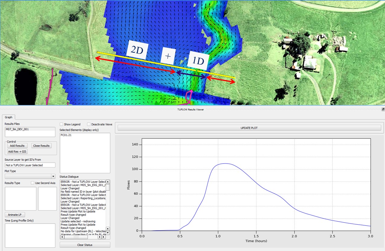
Figure 11.5: Example of the QGIS TUFLOW Plugin for a Reporting Location
11.3.4 Structure Output
The Structure Reporting feature outputs time-series and summary data for single and grouped structures. 1D and 2D structures are all output together to give a complete set of results. The summary output at the flood peak also produces the flow split between below and above deck, along with other information such as the head drop. The structure output is particularly useful in the reporting of hydraulic structure flows and afflux.
Structures are classified according to the following logic:
1D Structures:
- 1D structures that are in parallel (i.e. two structures that link to the same upstream and downstream nodes) are automatically grouped together and treated as a single structure for this output. The ID assigned to the group is the structure with the lowest bed elevation. Note that the directions of the digitised channels is important, that is, to form a group all channels must be digitised in the same direction.
- For 1D structures that have no parallel 1D structures, these are also included in the output so as to provide a complete set of results for all 1D structures.
- The flow split between below and above deck is based on the structure geometry, except weirs contributing to the below deck flow and/or above deck flow, depending on the configuration.
2D and 1D/2D Structures:
- To create a structure output that includes 2D flow, and optionally any 1D structures, the “QS” PO line is digitised in a 2d_po layer (see Section 11.3.2.1). All 2D flow across this line and any 1D structures that intersect this line are grouped together. The 1D structure’s 1d_nwk line does not have to snap with the QS line; they only have to cross over each other. The ID assigned to the structure output group is the 2d_po QS Label (see Table 11.10).
- If the 2d_po QS line selects cell sides that are modified by the Layered Flow Constriction or 2D Bridge feature, the summary output will split the flow into a below and above “deck” component based on Layers 1 to 2 being below “deck” and Layer 3 and 4 above.
- 2d_po HU and HD lines or points can be used to define the upstream and downstream water levels of the structure. HU objects should be located upstream of the structure and HD downstream. The average 2D water level along a line object will be used to populate the upstream and downstream water level data in the output. Lines can have more than two vertices (i.e. polylines are accepted). To associate the HU and HD objects with the QS line, all three (QS, HU and HD) must have the same ID for the 2d_po Label attribute Label (see Table 11.10). If a QS line has no HU and/or HD objects associated with it, output that cannot be produced, such as the water level drop across the structure, is given a -99999 value in the _SHmx.csv output file described below. HU and HD inputs are necessary for 2d_lfcsh and 2d_bg bridges.
An example model of the structure output for a bridge represented by a 2d_lfcsh is available in the 2D Structures Example Model Dataset on the TUFLOW Wiki.
The structure output is located in the plot/csv folder and includes:
- _SQ.csv file that contains time-series data of the flow through the structure. This file is similar to other time-series .csv output, but it only contains 1D and/or 2D structures as described above.
- _SHmx.csv file that contains a summary of each structure when the upstream water level reached its maximum. To generate this output the flow and other information is tracked every timestep for grouped structures. The output columns include: flow, area and average velocity for below and above deck; total flow, area and average velocity for the whole structure; upstream and downstream water levels; the head drop across the structure (i.e. upstream minus downstream water level); and the time these data were recorded (e.g. the time the upstream water level peaked).
- Time-series output for the upstream and downstream water levels are available through the 1d_H.csv, 2d_HD.csv and 2d_HU.csv files. Note that for the 2d_HD.csv and 2d_HU.csv files, if all 2D cells are dry a -99999 is output.
See Section 15.3.3 for further information on plotting of grouped structure results.
Two structure group check files are output if a model contains any structure groups (either automatically created, or via a “QS” type line in a 2d_po layer). The check files are both .csv files as follows:
- <simulation name>_Str_Grp_All.csv, contains information for all structure groups, including single 1D structures.
- <simulation name>_Str_Grp_Multi.csv, contains information for structure groups that are comprised of more than one 1D channel or are generated from a 2d_po “QS” line.
For more information on the structure group check files, please see the TUFLOW Wiki Check Files Str Grp.