5.18 Model Output

5.18.1 Command Status

Required.

5.18.2 Description

TUFLOW FV supports a range of output types and formats to enable review and presentation of model results. Results may be output at discrete locations such as points, hydraulic structures and polyline cross-sections, or across the full model mesh for spatial mapping and visualisation. This section describes the available 2D HD simulation class output types including configuration of output blocks, spatial definition of output locations and assignment of output parameters.

Model outputs are configured using the following process.

1. Select the required output type(s) (Section 5.18.2.1)
2. Define the directory where output(s) are to be saved (Section 5.18.2.2)
3. For each output type create an output block (Section 5.18.2.3)
4. Define the spatial output locations and configure the block for the selected output type (Sections 5.18.4 to 5.18.7)

Guidance for viewing of results is provided as part of the TUFLOW eLearning resource. Instructions for accessing this resource are provided in Section 5.2.

5.18.2.1 Output Model Implementations

The output model implementations for the 2D HD simulation class are summarised in Table 5.73. Each output type is described with configuration examples in the following sub-sections. Restart file output is configured using standalone restart commands and is described separately in Section 5.18.10.

Table 5.73: Output Model Implementations

Ouptut Type	Description
Mesh	Mesh output at all model cells. Also commonly referred to as ‘map output’ or ‘sheet output’.
Point	Cell output defined at discrete point locations.
Polyline	Flow integrated across discrete polylines (nodestrings).
Structure	Flow through hydraulic structures.
Mass Balance	Calculated model mass conservation outputs.
Mass	Total model volume output. It is a subset of the mass balance output and may be used if only total water volume diagnostic output is required.
Transport File	Writes a NetCDF file containing depth and velocity fields. This output file can subsequently be read in an advection dispersion simulation class model as a transport boundary condition.
Restart File	Write a binary output file that saves hydrodynamic variables that can be used as initial condition for a subsequent simulation.

5.18.2.2 Output Directories

Output files are written to directories defined by the user as listed in Table 5.74. These directory commands only need to be specified once in the control file and apply to all output blocks unless redefined later in the file.

Table 5.74: Output Directories

Command	Description
Output Dir	Required - Defines the directory where model results are saved. ‘Output Folder’ is also accepted.
Log Dir	Optional - Sets the model log directory.
Write Check Files	Optional - Writes model GIS check files to the specified directory.

! Model Output Directories
Output Dir == ..\results ! Result output directory
Log Dir == log ! Log and diagnostics directory
Write Check Files == ..\check ! Directory for GIS check files

5.18.2.3 Output Block

An output block defines the type and configuration of model result outputs.

The general form is:

! Defines the output type (e.g. Mesh, Points, Profiles)
Output == output_format

  …output_block_commands… ! Commands valid for the selected output type

End Output ! Terminates the output block

Where:

• Output == indicates the start of an output block
• output_format is a keyword selecting the output type or file format. The available output formats for each output type are defined in Sections 5.18.4 to 5.18.9
• output_block_commands are any commands that reside within the output block and are used to configure the output
• End Output closes the output block

The available 2D HD simulation class output block commands are described in Table 5.75.

Table 5.75: Output Block Commands

Command	Description
Output	Required - Defines the beginning of the output block and the result output format.
Output Interval	Required - The default (0.0 s, every model timestep) should be overridden for general use.
Output Parameters	Conditional - Required for points and mesh output types. Sets the model result output, for example water level, depth, velocity etc.
Read GIS PO	Conditional - Required for points model output. GIS layer that contains the location of the points.
Start Output	Optional - Defines the start time of the model output. If not specified, uses the model Start Time.
Final Output	Optional - Defines the final output time of the model output. If not specified, uses the model End Time.
Suffix	Optional - Enables multiple results of the same output format to be saved from the same simulation. Appends the suffix onto the result file name to ensure each result file name is unique.
Exact Timestep	Optional - Outputs the result at the exact computational timestep.
Output Compression	Optional - Enable or disable file compression for outputs in NetCDF file format (NetCDF, Transport, Profile).
Output Statistics	Optional - Track minimum or maximum map output values on a user-specifed Output Statistics dt.
Output Statistics dt	Optional - Sets the interval to track map output statistics.
End Output	Required - Defines the end of an output block.

5.18.2.3.1 Output Parameters

Map output parameters are model variables or diagnostic model results such as water level or flow velocity. Table 5.76 lists the available Output Parameters for the 2D HD simulation class. User specified output parameters are only required for points and mesh output types. All other output types report automatically configured output parameters.

Table 5.76: Output Parameters - 2D HD Simulation Class

Ouptut Parameter	Description	Units (Metric,Imperial)
H	Water surface elevation.	mRL, ftRL
D	Water depth.	m, ft
V	Velocity vector and magnitude.	m/s, ft/s
VMAG	Velocity magnitude only.	m/s, ft/s
TAUB	Bed shear stress.	N/m2, lbf/ft2
TAUS	Surface shear stress.	N/m2, lbf/ft2
ZB	Cell centre bed elevation.	mRL, ftRL
Z0	Depth x velocity product.	m2/s,ft2/s
HAZARD_Z1	Hazard catergories as outlined in the Australian NSW Floodplain Management Manual.	NA
HAZARD_ZAEM1	Hazard categories as outlined by Australian Emergency Management Institute.	NA
HAZARD_ZQRA	Hazard categories as outlined for the Queensland Reconstruction Authority.	NA
MSLP	Mean sea level pressure (hPa).	hPa, NA
W10	10 m wind speed vector (m/s).	m/s, NA
PRECIP	Precipitation rate (m/day).	m/day, NA
WVHT	Significant wave height (m).	m, NA
WVPER	Peak wave period.	s, NA
WVDIR	Mean wave direction.	degrees cartesian, NA
WVSTR	Wave stress vector.	N/m2, NA
TURB_VISC	Turbulent eddy viscosity.	m2/s,ft2/s

5.18.3 Mesh

Mesh outputs contain result output at every cell in the model. Mesh outputs are commonly used for statistical analysis, mapping, result checking and visualisation. The general process for specifying mesh output is as follows.

1. Choose a mesh output format from Table 5.77
2. Configure one or more output blocks
   
3. Select from the output parameters as listed in Section 5.18.2.3.1
4. Configure the output block with the required output interval
5. Optionally include statistics tracking Section 5.18.3.1

Examples for each recommended mesh output format are provided below.

Table 5.77: Recommended Mesh Output Formats

Ouptut Format	Description
NetCDF	Recommended for use with the QGIS TUFLOW Plugin. Supported by the TUFLOW FV Python Toolbox, and TUFLOW FV MATLAB Toolbox.
XMDF	Recommended for use with Aquaveo SMS.

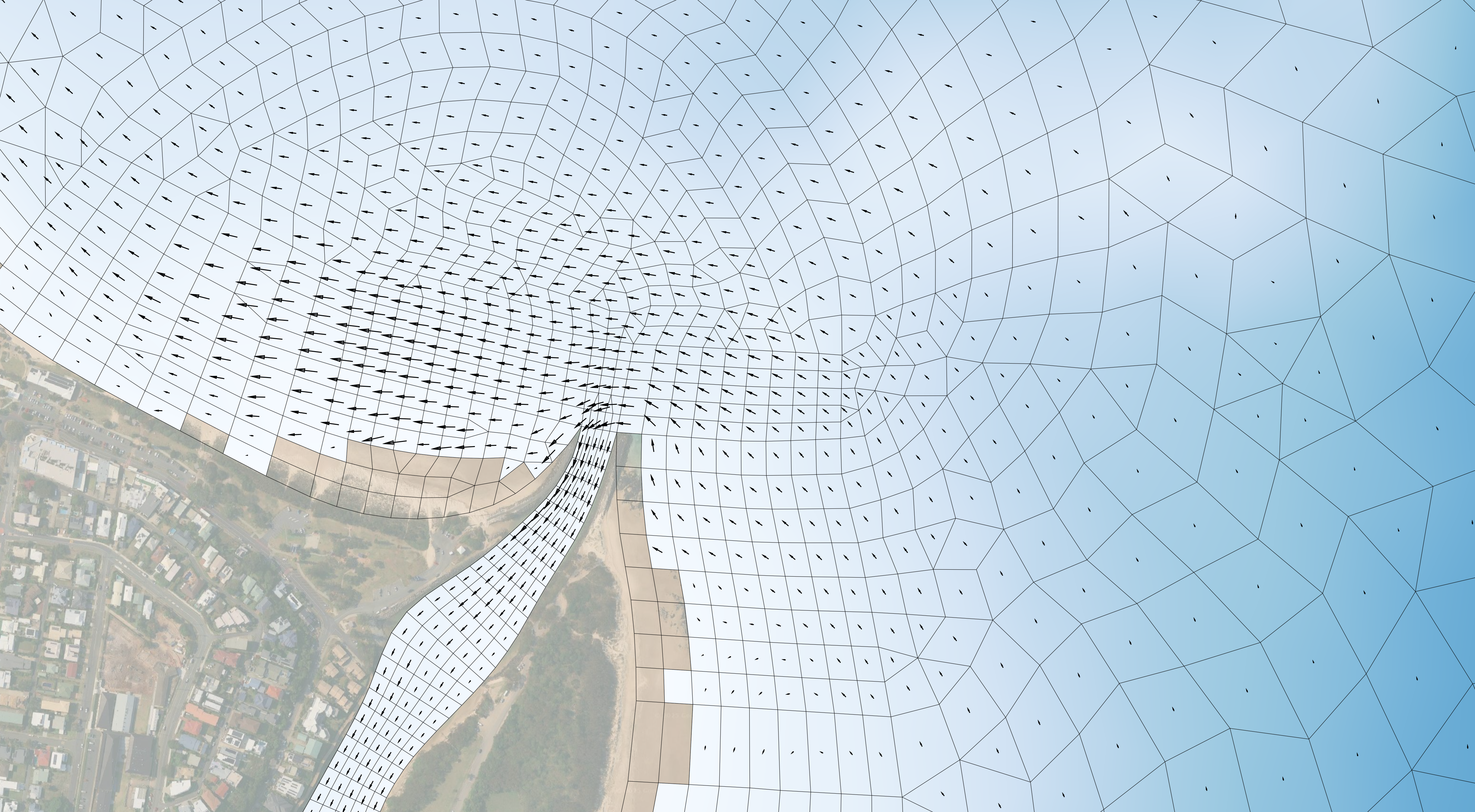
Figure 5.22: Depth Output With Overlaid Velocity Vectors

Example (NetCDF mesh output format).

! NetCDF mesh output format
Output == netcdf
  Output Parameters == h, d, v ! Water level (mRL or ft), depth (m or ft), velocity (m/s of ft/s)
  Output Interval == 900. ! (s)
End Output

Example (XMDF mesh output format).

! XMDF mesh output format
Output == xmdf
  Output Parameters == h, d, v ! Water level (mRL or ft), depth (m or ft), velocity (m/s of ft/s)
  Output Interval == 900. ! (s)
End Output

5.18.3.1 Statistics

The Output Statistics output block command outputs tracked minimum and maximum statistics over the duration of a simulation at a user specified interval set using the Output Statistics dt output block command. A comparison of NetCDF mesh velocity output at a timestep (left) and maximum of all timesteps (right) is shown in Figure 5.23.

More advanced statistical analysis is available via the TUFLOW FV Python Toolbox and TUFLOW FV MATLAB Toolbox.

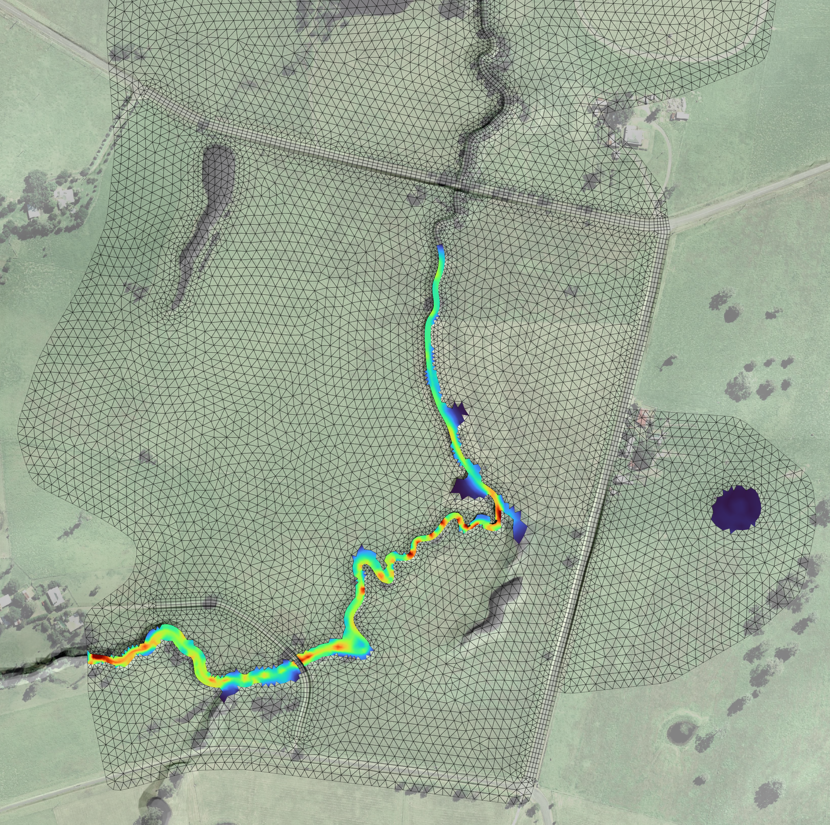
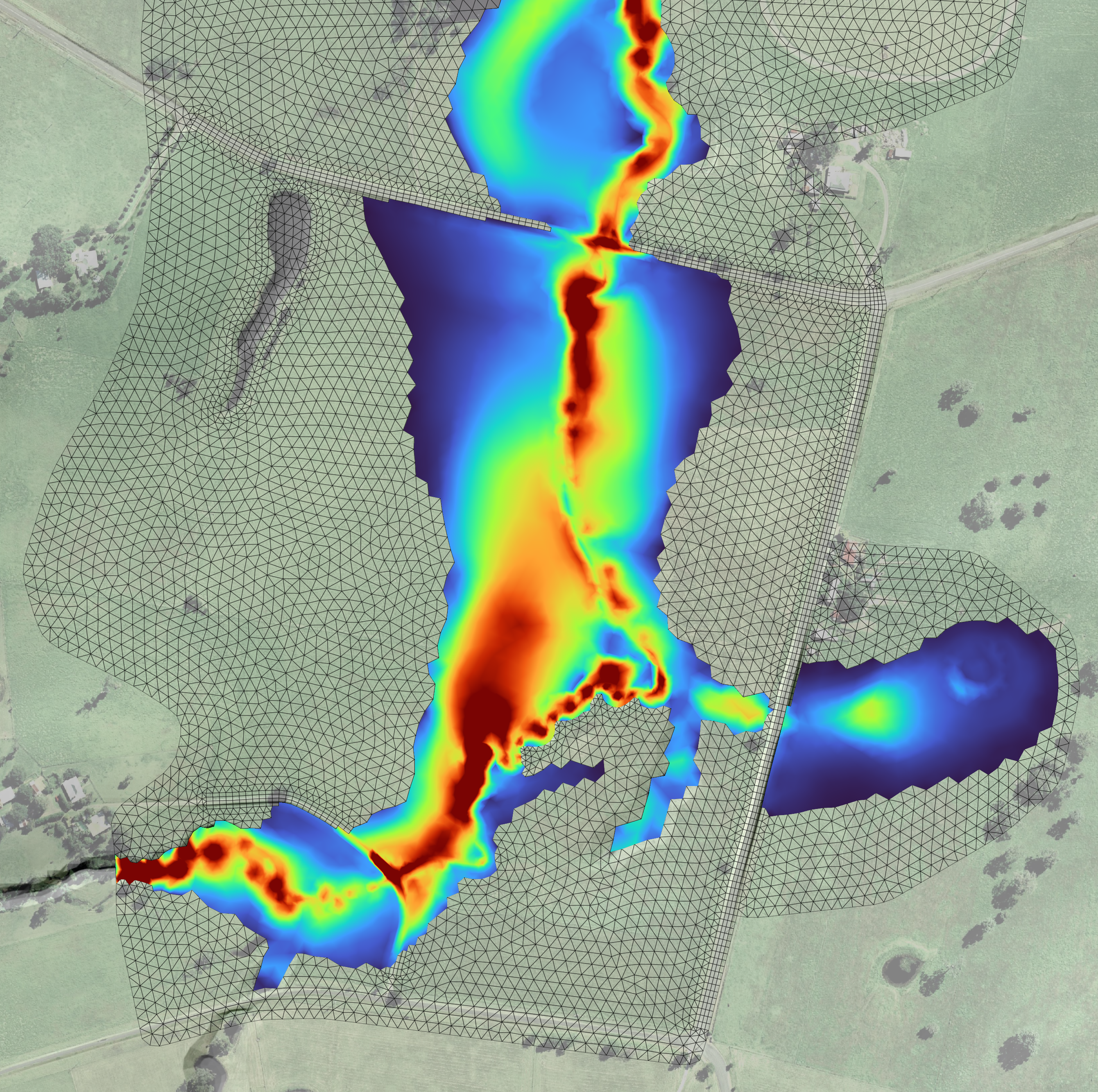
Figure 5.23: Maximum velocity over time

Example (NetCDF mesh output format with statistics).

! Mesh statistics output
Output == netcdf
  Output Parameters == h, d, v ! Water level (mRL or ft), depth (m or ft), velocity (m/s of ft/s)
  Output Interval == 900. ! (s)
  Output Statistics == min, max ! Track min/max
  Output Statistics dt == 1 ! (s) stat timestep
End Output

Example (XMDF mesh output format with statistics).

! Mesh statistics output
Output == xmdf
  Output Parameters == h, d, v ! Water level (mRL or ft), depth (m or ft), velocity (m/s of ft/s)
  Output Interval == 900. ! (s)
  Output Statistics == min, max ! Track min/max
  Output Statistics dt == 1 ! (s) stat timestep
End Output

5.18.4 Point

The point output type generates comma delimited text file (.csv) timeseries at discrete cell centre locations. One or more points may be reported within a single simulation.

Output .csv files are written to the Output Dir (Section 5.18.2.2) and use the naming convention <fvc_name>_POINTS.csv. For example, the simulation file CC_001.fvc will produce point output as CC_001_POINTS.csv.

Output point locations are defined using GIS layers read by the Read GIS PO command. This command reads 3d_po_ layers and empty template layers are generated during model initialisation (Section 5.2). Each 3d_po_ point must include a populated Label attribute as described in Table 5.78. Figure 5.24 shows output point locations from two example 3d_po_ layers. Yellow points represent offshore ADCP monitoring sites and red points indicate onshore meteorological logger locations.

Table 5.78: 3D PO (3d_po_) Attribute Description

Attribute Name(s)	Description	Type
Type	Reserved for future use (Not used)	Character
Label	Name of the point.	Character
Comment	Optional user comment.	Character
Vert_min	3D Vertical averaging override. Not applicable to the 2D HD simulation class.	Float
Ver_max	3D Vertical averaging override. Not applicable to the 2D HD simulation class.	Float

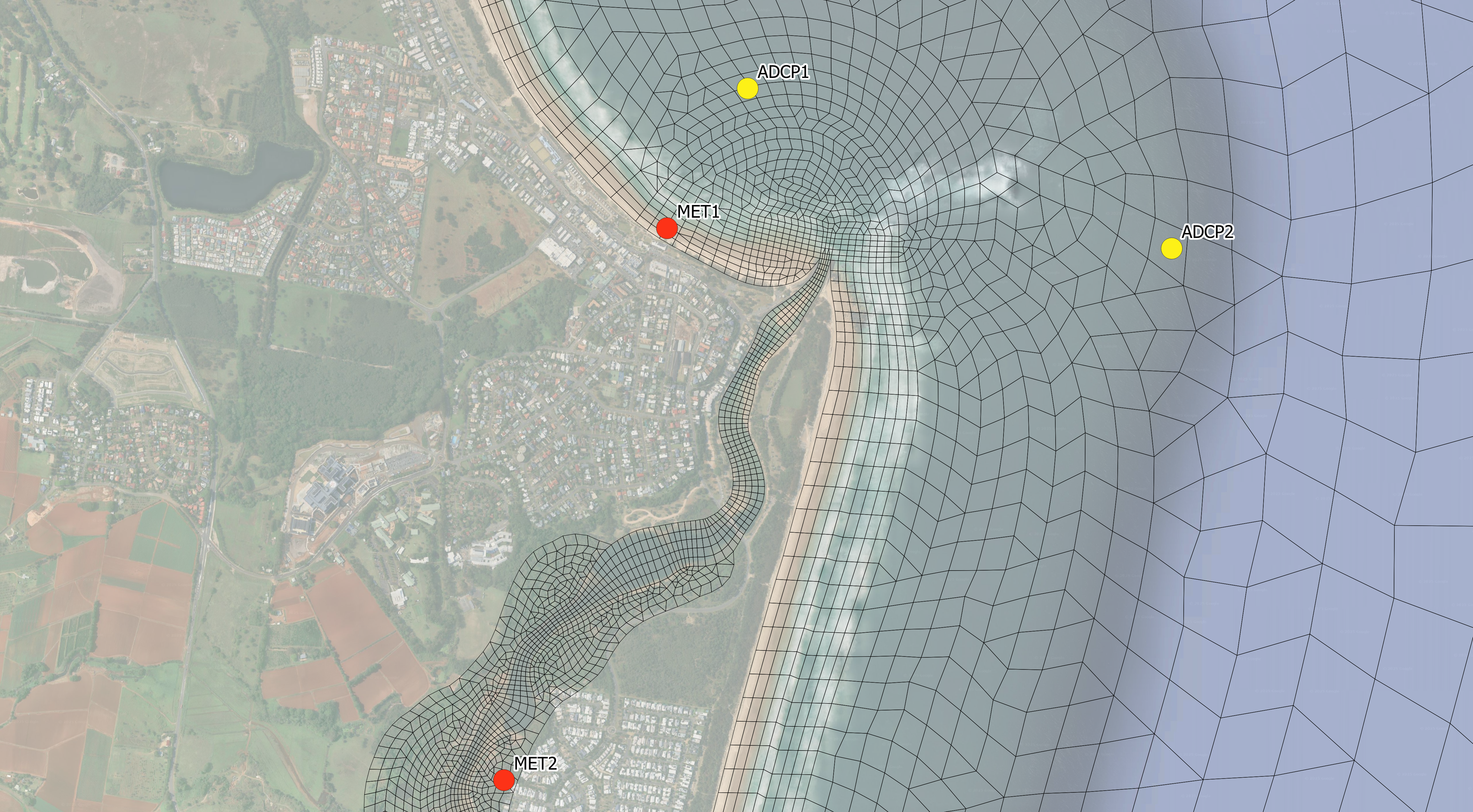
Figure 5.24: Point Output Locations

The point output type is specified by setting the first argument in the output block to points. Configuration requires specifying the output interval and the desired output parameters. Supported output parameters and their units are provided in Table 5.76.

Two examples output blocks are shown below. The first reports water level, depth, and velocity at the ADCP points, resulting in the output shown in Figure 5.25. The second reports wind speed and mean sea level pressure at the meteorological logger points, resulting in the output shown in Figure 5.26.

! ADCP Calibration Points
Output == Points ! CSV timeseries at each output point
  Read GIS PO == ..\model\gis\3d_po_ACDPs_001_P.shp ! Point locations
  Output Parameters == h, d, v ! Water level (mRL or ft), depth (m or ft), velocity (m/s of ft/s)
  Output Interval == 900. ! (s)
End Output

! Meteorological Boundary Comparisons To Measurements
Output == Points ! CSV timeseries at each output point
  Read GIS PO == ..\model\gis\3d_po_MetObs_001_P.shp ! Point locations
  Output Parameters == W10, MSLP ! Wind speed (m/s), mean sea level pressure (hPa)
  Output Interval == 3600. ! (s)
  Suffix == MET ! Appends _MET to output to avoid overwrite of HD outputs
End Output

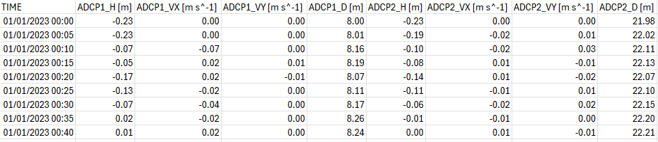
Figure 5.25: Point Output Timeseries From CC_001_POINTS.csv

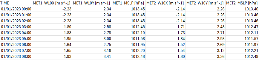
Figure 5.26: Point Output Timeseries From CC_001_POINTS_MET.csv

5.18.5 Polyline

The polyline output type (also referred to as flux output) generates comma delimited (.csv) timeseries of net flow across each nodestring feature in the model. This includes nodestrings associated with open boundary definition, hydraulic structure connections and user defined monitoring locations.

Output files are written to the Output Dir (Section 5.18.2.2) and follow the naming convention _FLUX.csv. For example, the simulation file CC_001.fvc will produce CC_001_FLUX.csv.

Polyline output locations (Figure 5.27) are defined using the Read GIS Nodestring command which reads 2d_ns_layers. Digitising flow monitoring polylines uses the same approach as nodestring structure connection types (Section 5.17.2.2.1). For correct sign convention polylines should be digitised from right to left when looking in the downstream direction.

Polyline timeseries output is specified by setting Output == Flux on the first line of the output block (Example provided below). No output parameters are required. The output variable (See Table 5.79) is fixed to net flow and cannot be modified.

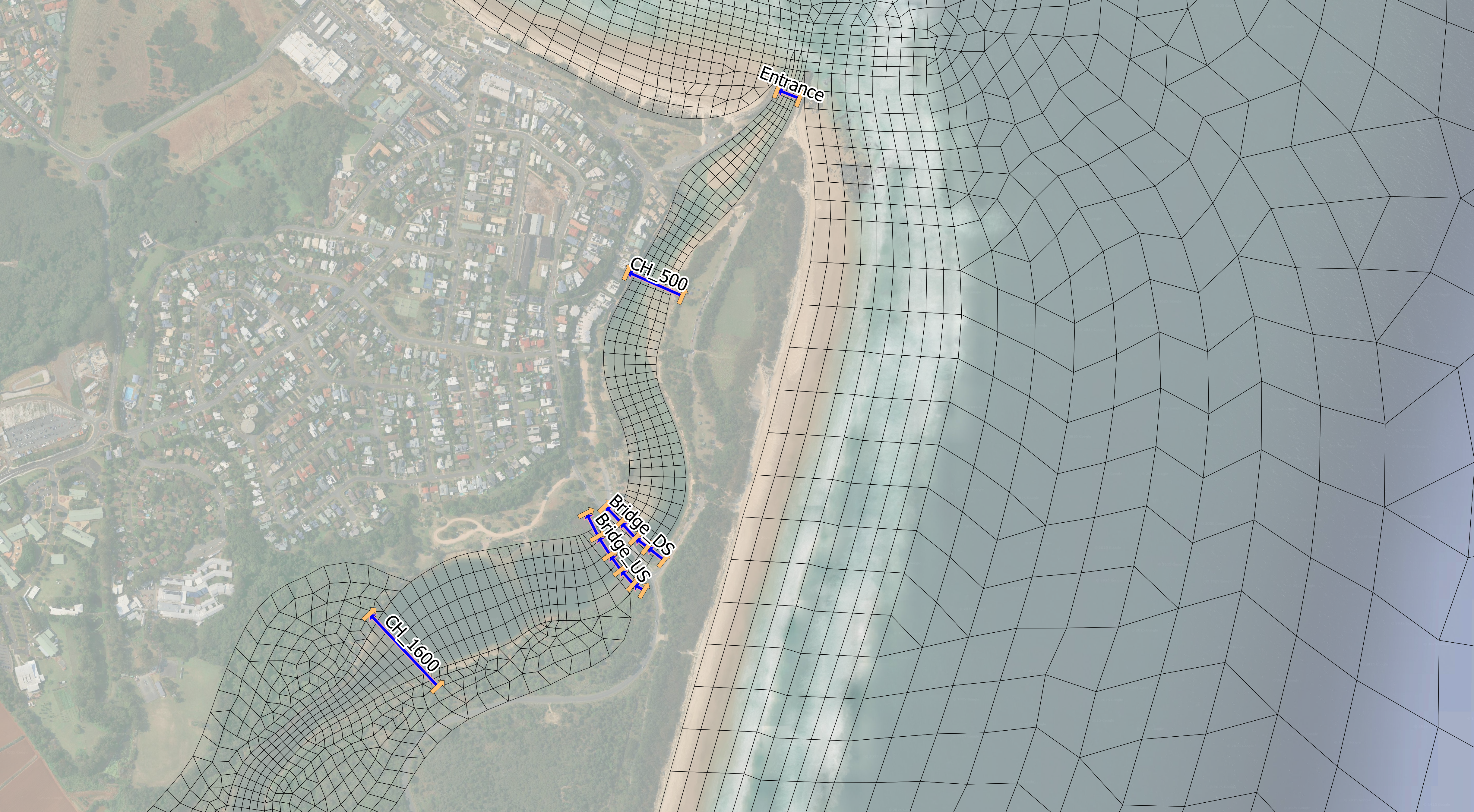
Figure 5.27: Polyline Output Locations

Table 5.79: Flux Output Variables

Output	Description	Units (Metric,US Customary)
FLOW	Net flow across the nodestring.	m3/s, ft3/s

! Location of Flux Polylines
Read GIS Nodestring == ..\model\gis\2d_ns_Monitoring_001_L.shp

! Output Flux Cross/Long Sections
Output == Flux ! Net flux across each nodestring
  Output Interval == 300. ! (s)
End Output

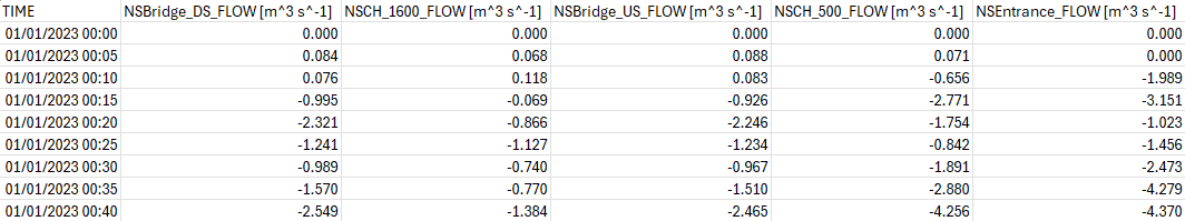
Figure 5.28: Net Flow Timeseries From CC_001_FLUX.csv

5.18.6 Structure

The structure output type (also referred to as structflux output) generates comma delimited (.csv) timeseries of flow (in units of \(m^3/s\) or \(ft^3/s\)) through hydraulic structures.

Output files are written to the Output Dir (Section 5.18.2.2) and follow the naming convention _STRUCTFLUX.csv. For example, the simulation file CC_001.fvc will produce CC_001_STRUCTFLUX.csv.

If the Name structure block command is populated the csv output column will use the name as a label. Otherwise the column header will be labelled STRUCTURE_N_FLOW where N is the order that the structure block appears in the .fvc file. For example, STRUCTURE_1_FLOW is the first structure block encounter in the .fvc file as shown in Figure 5.29.

There is no need to specify output parameters for structflux output, all relevant outputs are automatically generated (see Table 5.80). )

Table 5.80: Flux Output Variables

Output	Description	Units (Metric,US Customary)
FLOW	Flow through the structure.	m3/s, ft3/s

! Structure flux output
Output == structflux
  Output Interval == 300. ! (s)
End Output

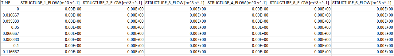
Figure 5.29: Structure Flow Timeseries From CC_001_STRUCTFLUX.csv

5.18.7 Mass Balance

Mass balance output generates comma delimited (.csv) time series of accumulated fluxes and balance diagnostics for each simulated quantity for commonly used boundary conditions. These outputs are useful for checking domain scale conservation and understanding system turnover dynamics. Mass balance output is not supported when using the Cartesian (US Customary Units) coordinate reference frame implementation.

Output files are written to the Output Dir (Section 5.18.2.2) using the naming convention <fvc_name>_MASSBALANCE_<quantity_name>.csv. For example, the volume balance file for River_001.fvc is River_001_MASSBALANCE_VOLUME.csv.

There is no need to specify output parameters for mass balance output. The key outputs reported for each quantity are summarised in Table B.4.

! Accumulated volume and mass balance
Output == massbalance
  Output Interval == 900. ! (s)
End Output

Output csv header code definitions, units, and interpretation guidance are provided in Appendix B.11.1.

5.18.8 Mass

Mass output tracks the water volume, mass and potential energy in the model. There is no need to specify output parameters for mass output. Mass output is not supported when using the Cartesian (US Customary Units) coordinate reference frame implementation.

Table 5.81: Mass Output Variables

Output	Description	Units (Metric only )
Volume	Total water volume in the model.	m3
Water Mass	Total water mass in the model.	tonnes
Potential Energy	Total potential energy in the model.	GJ

! Global volume tracking
Output == mass
  Output Interval == 900. ! (s)
End Output

5.18.9 Transport File

Transport files are generated from an existing 2D TUFLOW FV simulation as model output. The file stores hydrodynamic state variables and may subsequently be read in a new simulation to provide prescribed hydrodynamic forcing.

Transport output stores cell volume (depth) and depth averaged momentum components (X-momentum and Y-momentum) at a user defined interval. These fields may later be read using a Transport boundary condition within an Advection Dispersion simulation (See Section 7.11.10).

This workflow is commonly applied where multiple tracer, sediment transport, particle tracking or water quality scenarios are run using identical hydrodynamic conditions.

! Output Transport HD file
Output == Transport
  Output Interval == 900. ! (s)
End Output

5.18.10 Restart File

Restart files are written from a 2D HD simulation to store the hydrodynamic state variables required to resume a 2D HD simulation. The file may subsequently be read by a new simulation to initialise water level, depth and momentum fields, enabling continuation of a previous run or staged model workflows. The reading of restart files as initial conditions is described in Section 5.15.5.

Restart files are written using standalone restart commands. Unlike other model outputs, restart files are not configured within an Output Block.

The standalone restart commands are listed in Table 5.82.

Table 5.82: Restart Commands

Command	Description
Write Restart dt	Optional - Writes a restart file (.rst) to the log directory location at the time interval specified.
Restart Overwrite	Optional - Switch to overwrite the restart file at the time interval specified using the Write Restart dt command or create a series of restart files for each timestep:

The example below specifies periodic writing of restart data.

! Write Restart File
Write Restart dt == 24.0 ! Interval (hours) for writing restart data
Restart Overwrite == 1 ! Enable overwrite mode (1: overwrite, 0: don’t overwrite)

Write Restart dt specifies the interval in hours at which restart data are written. Restart Overwrite controls whether successive restart files overwrite the previous file or are written as separate files. If overwrite mode is enabled only a single restart file representing the most recent write time is retained. If disabled, a restart file is written at each specified interval.

5.18.11 Checks and Logs

Several diagnostic style outputs are produced by TUFLOW FV to assist in debugging and simulation optimisation.

5.18.11.1 Check Files

Check files are written when the Write Check Files command is issued with a folder path argument.

Write Check Files == ..\check ! Directory for GIS check files

These files are GIS vector files and summarise the mesh, nodestings, boundary conditions, z line and sa inputs. One file is produced for each and presents the sum total of all specifications or manipulations applied to a simulation across one to many commands. For example, a boundary condition check file will show all the locations of boundary conditions in one file, irrespective of how many BC block commands have been issued.

Check files are described, and their attributed explained, within a dedicated TUFLOW FV Wiki page.

5.18.11.2 Log File

A log file is written when the Log Dir command is issued with a folder path argument. The interval that the log file is updated during a simulation can be configured using the Screen/Log Display Interval.

Log Dir == log ! Log and diagnostics directory
Screen/Log Display Interval == 300. ! {300.} log_dt (s)

This file echoes the .fvc and provides error messaging, timestep related information and other diagnostic data. This file is therefore important for identifying data input issues and troubleshooting the model.

5.18.11.3 Timestep Files

Files that describe the overall CFL behaviour of each cell face are written at the end of each simulation, in the same location as the log file. These are useful in quickly identifying which cell faces (if any) are potentially unnecessarily slowing down simulations (i.e. are reducing the overall simulation timestep to meet CFL conditions, see Section 5.7 and Appendix B.4.5). These often occur in locations with small cells that may have been accidentally built. One csv file is produced for each of the internal and external CFL performance, and average and minimum timestep information for each cell face is provided. Faces that are constraining the timestep can be easily identified by sorting the output csvs in a spreadsheet application - the smallest timesteps will be at the top (or bottom) of the sorted list, alongside the corresponding cell face ID and geospatial coordinates.

Guidance on interrogating these files is provided within a dedicated TUFLOW FV Wiki page.