7.7 Atmospheric Heat Exchange
7.7.2 Description
A range of models are available to support simulation of heat and potentially its impact on hydrodynamics via baroclinic (temperature density driven) processes (see Section 7.3.5). This capability is typically deployed where thermal stratification or water quality dynamics are of interest.
The core atmospheric heat exchange components in TUFLOW FV are conceptualised in Figure 7.1 as follows.
- Incoming (water heat gain, positive quantities)
- Incident shortwave (visible) solar radiation
- Incident longwave (infrared) radiation
- Outgoing (water heat loss, negative quantities)
- Reflected shortwave (visible) solar radiation
- Reflected longwave (infrared) radiation
- Longwave radiation emitted by the water
Both shortwave and longwave radiation can be reflected by the model bed.
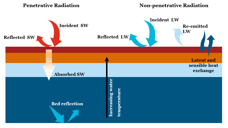
Figure 7.1: Atmospheric Heat Exchange Conceptual Diagram
Atmospheric heat exchange is enabled via the command
Four models are required if atmospheric heat exchange is simulated as per Table 7.9. One or more may be individually parameterised. If no parameters are set for a given model then the model is deployed with default settings.
The TUFLOW FV Get Atmos tool can be used to source the atmospheric boundary conditions (see Section 7.11.6) required to run the default combination of atmospheric heat exchange models.
| Atmospheric Heat Exchange Component | Description |
|---|---|
| Shortwave Radiation Model | Estimates incoming shortwave (penetrative) radiation at the water surface. |
| Longwave Radiation Model | Estimates net longwave (non-penetrative) radiation exchange at the water surface. |
| Latent Heat Model | Computes latent heat exchange flux components and transfer terms. |
| Sensible Heat Model | Computes sensible heat flux using the selected coefficient method. |
7.7.3 Shortwave Radiation Model
Two models are available to estimate surface shortwave radiation (in W/m\(^2\)) entering the top of the simulated water column. The
| Model Implementation | Description |
|---|---|
| Jacquet | Default shortwave implementation that applies albedo to specified shortwave boundary data. Requires short wave radiation input. |
| Zillman | Clear sky shortwave implementation with cloud cover correction. Requires air temperature and relative humidity, with optional cloud cover. |
| Command | Description |
|---|---|
| Shortwave Radiation Model | Optional - Selects the shortwave radiation implementation. If not specified the default Jacquet is used. |
| Shortwave Radiation Albedo | Optional - Sets the local shortwave radiation albedo (reflectivity). |
| Shortwave Radiation Fractions | Optional - Sets the fraction of total incoming shortwave radiation into Photosynthetically Active Radiation (PAR), Ultraviolet A (UVA), Ultraviolet B (UVB) and Near Infrared (NIR), in that order. |
| Shortwave Radiation Extinction Coefficients | Optional - Sets the extinction coefficient for each shortwave radiation fraction (PAR, UVA, UVB and NIR). |
| Shortwave Radiation Bed Absorption | Optional - Sets the proportion of shortwave radiation that is absorbed on reaching the bed. |
7.7.3.1 Jacquet
This model is the default. It adjusts user specified shortwave radiation boundary data using albedo, following Jacquet (1983). Albedo is computed using Equation (B.49). Incoming surface shortwave radiation is computed by multiplying user specified shortwave radiation boundaries by computed albedo as per Equation (B.50). This model is typically used when shortwave radiation data from a third party model is available.
7.7.3.2 Zillman
This model estimates incident shortwave radiation under clear sky conditions with a cloud cover correction following Zillman & Commonwealth Bureau of Meteorology (Australia) (1972).
Air temperature, relative humidity and cloud cover are used to estimate incoming shortwave radiation, as described in Appendix B.5.1.2. If cloud cover is not specified, clear sky conditions with no cloud correction are assumed. This model is typically used when shortwave radiation data from a third party model is unavailable.
7.7.4 Longwave Radiation Model
Five models are available for estimating net longwave radiation (in W/m\(^2\)). The
| Model Implementation | Description |
|---|---|
| Net | Uses specified net longwave radiation directly. Requires net downward longwave radiation. |
| Incident (Direct) | Default implementation using specified incident longwave radiation with albedo reflection and emitted longwave calculation. Requires incident downward longwave radiation. |
| Incident (TVA) | Computes incident longwave radiation from air temperature with cloud cover correction. Requires air temperature and cloud cover. |
| Incident (Zillman) | Variant of the TVA approach with outgoing longwave estimation based on air-water temperature difference. Requires air temperature and cloud cover. |
| Incident (Chapra) | Computes incident longwave radiation from air temperature and humidity with reflectivity and emitted longwave terms. Requires air temperature and relative humidity. |
| Command | Description |
|---|---|
| Longwave Radiation Model | Optional - Selects the longwave radiation implementation. If not specified the default Incident (Direct) is used. |
| Longwave Radiation Albedo | Optional - Sets the local longwave radiation albedo (reflectivity). |
| Water Emissivity | Optional - Sets the emissivity of water. |
7.7.4.1 Net
This model accepts estimates of user specified net longwave radiation only without change. This model might be used where net longwave radiation data from a third party model is readily available.
7.7.4.2 Incident (Direct)
This model is the default. Specified incident longwave radiation is modified by a computed longwave radiation albedo and outgoing longwave radiation emitted by the water surface is calculated using water temperature and the Stefan-Boltzmann law. Net long wave radiation is then computed as the difference of these quantities, as described in Appendix B.5.2.2. This model might be used where incident longwave radiation data from a third party model is readily available.
7.7.4.3 Incident (TVA)
This model is the default. Specified incident longwave radiation is modified by a computed longwave radiation albedo and outgoing longwave radiation emitted by the water surface is calculated using water temperature and the Stefan-Boltzmann law. Net long wave radiation is then computed as the difference of these quantities, as described in Appendix B.5.2.3. This model might be used where incident longwave radiation data from a third party model is readily available.
7.7.4.4 Incident (Zillman)
This model is similar to Incident (TVA) but estimates outgoing longwave radiation using a combination of water and air temperatures, as described in Appendix B.5.2.4. This model might be used where incident longwave radiation data from a third party model is unavailable, but typical meteorological data are accessible.
7.7.4.5 Incident (Chapra)
This model is similar to Incident (TVA) and Incident (Zillman), estimating incident longwave radiation using a combination of air temperature and relative humidity following Chapra (2008), as described in Appendix B.5.2.5. This model might be used where incident longwave radiation data from a third party model is unavailable, but typical meteorological data are accessible.
7.7.5 Latent Heat Model
Latent heat flux calculations are performed after shortwave and longwave radiation fields are computed. Regardless of the selected model, all latent heat formulations compute the following, in order.
- Vapour pressures (two, in Pascals) and specific humidities (two, dimensionless), computed by one of two models
- Vapour pressure of water and specific humidity in atmospheric air, \(P_a\) and \(E_a\), respectively
- Vapour pressure of water and specific humidity due to the presence of surface water, \(P_w\) and \(E_w\), respectively
- Bulk aerodynamic latent heat transfer coefficient (J/kg), set by one model
- Latent heat of vaporisation (J/kg), set by one model
The following content is therefore sectioned accordingly.
7.7.5.1 Vapour Pressure and Specific Humidity
Two vapour pressure and specific humidity options are available, selected using the
| Model Implementation | Description |
|---|---|
| Magnus-Tetens | Default model for vapour pressure and specific humidity calculations. |
| Lowe and Reed | Alternative vapour pressure and specific humidity model based on Lowe and Reed. |
| Command | Description |
|---|---|
| Latent Heat Model | Optional - Selects the vapour pressure and specific humidity model. If not specified the default Magnus-Tetens is used. |
| Vapour Pressure Salinity Parameters | Optional - Applies salinity correction parameters in specific humidity calculations. |
7.7.5.1.1 Magnus-Tetens
This model is the default. Specified air temperature and relative humidity are used to compute vapour pressures \(P_a\) and \(P_w\) following Magnus-Tetens (see Appendix B.5.3.1.1). These are then used to compute \(E_a\) and \(E_w\), respectively.
A correction may be applied to the calculation of specific humidity in the presence of water if that water contains dissolved salt. This can be set as follows.
7.7.5.1.2 Lowe and Reed
This model uses specified air temperature and relative humidity to compute vapour pressure \(P_a\) and \(P_w\) following Lowe (1977) and Reed (1977) (see Appendix B.5.3.1.2). These are then used to compute \(E_a\) and \(E_w\), respectively.
A correction may be applied to the calculation of specific humidity in the presence of water if that water contains dissolved salt (see syntax example in Section 7.7.5.1.1).
7.7.5.2 Bulk Aerodynamic Latent Heat Transfer Coefficient
Two bulk aerodynamic latent heat transfer coefficient models are available. Supported implementations are summarised in Table 7.16. Commands are summarised in Table 7.17.
| Model Implementation | Description |
|---|---|
| Constant | Default model with a constant bulk aerodynamic latent heat transfer coefficient. |
| Kondo | Computes the bulk aerodynamic latent heat transfer coefficient dynamically through Kondo wind stress with atmospheric stability. |
| Command | Description |
|---|---|
| Wind Stress Model | Conditional - Required as 3 (Kondo) when the Kondo bulk latent heat coefficient model is used. |
| Atmospheric Stability | Conditional - Required as 1 (ON) if using the Kondo bulk latent heat coefficient model. Includes the influence of air column stabilty in the calculation of the bulk transfer coefficient. Not used for the Constant bulk latent heat coefficient model. |
| Bulk Latent Heat Coefficient | Optional - Alters the bulk latent heat coefficient when using the Constant model. The default coefficient is a well established value that would require considerable justification to alter. |
7.7.5.2.1 Constant
This model is the default and sets a constant bulk aerodynamic latent heat transfer coefficient using the
This model is used when using Constant or Wu
7.7.5.2.2 Kondo
This model dynamically computes the bulk aerodynamic latent heat transfer coefficient using the Kondo wind stress model with atmospheric stability enabled (Equation (B.94)). It is invoked using the two commands (that also govern sensible heat calculations (Section 7.7.6.1.2 and wind stress calculations (Section 7.8)).
This will overwrite previous specifications (or the default) of the wind stress model.
7.7.5.3 Latent Heat of Vaporisation
By default, the latent heat of vaporisation (in J/kg) is constant and not user specifiable unless the Kondo model is activated.
7.7.5.3.1 Kondo
This model dynamically computes the latent heat of vaporisation as part of the Kondo wind stress model and is activated as described in Section 7.7.5.2.2. It does so using air temperature, as described in Appendix B.5.3.2.2, regardless of whether atmospheric stability has been activated.
7.7.6 Sensible Heat Model
Sensible heat flux calculations are performed after latent heat calculations. These require a bulk aerodynamic sensible heat transfer coefficient (in J/kg), see Appendix B.5.4.
7.7.6.1 Bulk Aerodynamic Sensible Heat Transfer Coefficient
Two bulk aerodynamic sensible heat transfer coefficient models are available. Supported implementations are summarised in Table 7.18. Commands are summarised in Table 7.19.
| Model Implementation | Description |
|---|---|
| Constant | Default model with a constant bulk aerodynamic sensible heat transfer coefficient. |
| Kondo | Computes the bulk aerodynamic sensible heat transfer coefficient through Kondo wind stress with atmospheric stability. |
| Command | Description |
|---|---|
| Wind Stress Model | Conditional - Required as 3 (Kondo) when the Kondo bulk sensible heat coefficient model is used. |
| Atmospheric Stability | Conditional. Required as 1 (ON) if using the Kondo bulk sensible heat coefficient model. Includes the influence of air column stabilty in the calculation of the bulk transfer coefficient. Not used for the Constant bulk sensible heat coefficient model. |
| Bulk Sensible Heat Coefficient | Optional - Alters the bulk sensible heat coefficient when using the Constant model. The default coefficient is a well established value that would require considerable justification to alter. |
7.7.6.1.1 Constant
This model is the default and sets a constant bulk aerodynamic sensible heat transfer coefficient. The default value of 0.0013 J/kg is a well accepted constant that would require considerable justification to alter.
7.7.6.1.2 Kondo
This model can be set to dynamically compute the bulk aerodynamic sensible heat transfer coefficient as part of the Kondo wind stress model with atmospheric stability enabled (Equation (B.99)). This model is invoked with two commands (that also govern latent heat calculations (Section 7.7.5.2.2 and wind stress calculations (Section 7.8)).
This will overwrite previous specifications (or the default) of the wind stress model.