Section 3 Process descriptions

Previous chapters have presented an overview of the architecture and capabilities of TUFLOW CATCH. This chapter presents the details of the processes that TUFLOW CATCH executes. It does not present the processes executed by either TUFLOW HPC or TUFLOW FV: these are detailed in the respective model user and science manuals, and relevant release notes here:

TUFLOW CATCH provides three primary functions:

Coordination of the execution of TUFLOW HPC and TUFLOW FV across a whole-of-catchment domain (Hydrology and Integrated configurations)
Automatic geolocation and writing of flow and concentration boundary conditions for TUFLOW FV (as the receiving water model), generated from TUFLOW HPC predictions (as the catchment model) (Hydrology and Integrated configurations)
Pollutant export and transport calculations within a catchment (Pollutant export and Integrated configurations)

The first of these is its core architectural capability and so is described in Section 2.3.1. The latter two are technical componentry of this architecture and so are detailed here in Sections 3.1 and 3.2, respectively.

3.1 Geolocation

Manually linking catchment and receiving water models can potentially be a time consuming and error prone process. When executed in configurations other than Pollutant export (see Section 1.3), TUFLOW CATCH undertakes this task automatically via a process of geolocation, whereby TUFLOW HPC cells that spatially coincide with either TUFLOW FV nodestring inflows (user nominated, see Section 4.5.4) or TUFLOW FV mesh cells are identified. These TUFLOW HPC cells are called transfer cells. Once identified, these transfer cells track the local surface and groundwater flow volumes and constituent masses predicted by TUFLOW HPC, and each transfer cell’s outflows are converted into timeseries and exported into the comma delimited (.csv) format expected by TUFLOW FV as boundary conditions. It is noted that:

Where the user has nominated a nodestring/s as transfer locations from TUFLOW HPC to TUFLOW FV, TUFLOW CATCH will write the corresponding TUFLOW FV boundary condition files as ‘Q’ types that include the transfer of momentum from TUFLOW HPC to TUFLOW FV. As such, these boundaries (and specifying the corresponding TUFLOW FV nodestrings) should be considered where channelised riverine inflows and the like are to be matched, i.e. where inflow momentum is important in controlling receiving water hydrodynamics
Where TUFLOW CATCH automatically geolocates non-nodestring transfer locations from TUFLOW HPC to TUFLOW FV, TUFLOW CATCH will write the corresponding TUFLOW FV boundary condition files as ‘QC’ types that exclude the transfer of momentum from TUFLOW HPC to TUFLOW FV. As such, these boundaries should typify non-channelised ‘lateral’ inflows where momentum transfer is less important in controlling receiving water hydrodynamics
Boundary data for TUFLOW FV is written with date (dd/mm/yyyy hh:mm:ss) format
TUFLOW HPC cells that are located within the TUFLOW FV mesh but are not transfer cells (e.g. lie well within the TUFLOW FV model mesh) are designated as deactivated within TUFLOW HPC and are not included in simulation

This automated selection of linkage cells is sufficiently robust to handle relative differences in mesh/grid resolution between TUFLOW HPC and TUFLOW FV, including cases where the TUFLOW HPC model is higher resolution than the (local) TUFLOW FV model mesh, and vice-versa. Some typical cases are presented in Figure 3.1.

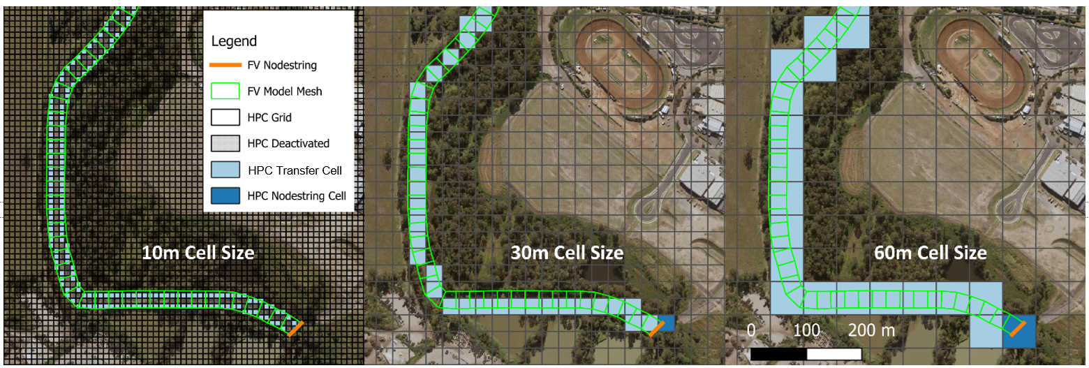
Figure 3.1: Examples of linkages under varying TUFLOW HPC and TUFLOW FV cell resolutions

After all mesh elements and boundary nodestrings are processed, any cells entirely within the TUFLOW FV mesh are deactivated from TUFLOW HPC computations - these locations within the overall model domain are simulated by TUFLOW FV.

The locations of the TUFLOW HPC transfer cells automatically geolocated by TUFLOW CATCH are reported in the TUFLOW HPC ‘hpc_transfer’ check file for review. The corresponding TUFLOW FV boundary condition locations are also reported in the TUFLOW FV ‘bc_check_P’ check files. An example of both is presented in Figure 3.2, with TUFLOW HPC and TUFLOW FV check file outputs on the left (brown squares) and right (red dots), respectively.

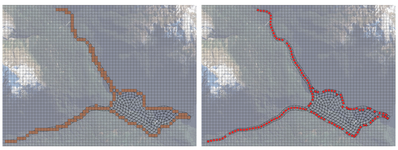
Figure 3.2: HPC transfer cell (left) and TUFLOW FV boundary cell (right) check file examples

The above geolocation process does not exclude or prevent the TUFLOW FV user from manually specifying additional boundaries to a TUFLOW FV model. For example, tidal or wastewater discharge (or other) boundaries can be specified by the user within the TUFLOW CATCH control file as per a normal TUFLOW FV model set up by specifying ‘bc’ blocks as required. TUFLOW CATCH will collect these manual (user defined) boundaries and all automatically geolocated boundaries and apply them to the execution of TUFLOW FV under TUFLOW CATCH.

An example of how this geolocation method supports transfer of water, concentrations and momentum is provided in Figure 3.3. The animation presents a catchment derived TUFLOW HPC flow originating from left of screen (and from the fixed grid domain) being transferred automatically into the (flexible mesh) TUFLOW FV domain, and then advected downstream to the right. Constituent concentrations vary from low (blue) to red (high).

Figure 3.3: Example of transferral of an inflow (from left to right) from TUFLOW HPC to TUFLOW FV. Omitted in pdf version

3.2 Pollutant export

TUFLOW CATCH supports the simulation of pollutant generation and associated surface (and optionally subsurface) transport within the catchment domain. It does so on a spatially varying basis via use of materials so that, in a manner analogous to hydraulic roughness calculations (that also use materials), pollutant export simulation is ultimately affected on a computational cell by computational cell basis. This obviates the need to make top-down lumped hydrologic or pollutant export related assumptions, and facilitates the solution of the equations of motion and solutes on a spatially and temporally resolved basis. \(\newcommand{\blockindent}{\hspace{0.5cm}}\)

Pollutant export simulation within TUFLOW CATCH allows for any of the following simulation methods per pollutant:

Constant. Specification of a constant concentration to be written to TUFLOW FV boundary conditions without numerical simulation in TUFLOW HPC. Examples include water quality constituents that are not meaningfully conceptualised as being liberated from a ground surface, such as dissolved oxygen, or
Timeseries. Specification of a time varying concentration, again to be written to TUFLOW FV boundary conditions without numerical simulation. Examples include water temperature
Material based. Specification of the following on a material by material basis, for a given pollutant:
- The computational pollutant export method to be used
- The parameters associated with the selected computational pollutant export method

Different pollutant export methods across the above options can be used within a single TUFLOW CATCH simulation for different pollutants. A given pollutant, however, should not have different material based pollutant export methods applied to it within a given simulation. Commands are provided in detail in Section 4, however an example of such a specification is provided following, with incomplete (…) parameter lists for brevity.

Constant POLLUTANT_A == 8.0
Time-series POLLUTANT_B == temptre

Material == ALL
  POLLUTANT_C,Method==method1,param1==100.0...
  POLLUTANT_D,Method==method2,param1==10.0...
  POLLUTANT_E,Method==method1,param1==0.17...
  POLLUTANT_F,Method==method2,param1==1.23...
  ...
End Material

Material == 1,4
  POLLUTANT_C,Method==method1,param1==43.0...
  POLLUTANT_E,Method==method1,param1==0.37...
  ...
End Material

Multiple constant and time-series pollutants can be specified (via individual command lines), and material blocks can be specified to apply to more than one material (the above example applies to ALL materials, then materials 1 and 4, for example). In a manner akin to specification of roughness in TUFLOW HPC, sequences of material blocks progressively spatially overwrite in the order presented. In the above example, materials 1 and 4 would therefore be interpreted as

Material == 1,4
  POLLUTANT_C,Method==method1,param1==43.0...
  POLLUTANT_D,Method==method2,param1==10.0...
  POLLUTANT_E,Method==method1,param1==0.37...
  POLLUTANT_F,Method==method2,param1==1.23...
  ...
End Material

Materials 2 and 3 would be as per the ALL specification above.

Different computational pollutant export methods can be assigned to different pollutants within a single material block. The same computational pollutant export method should be assigned to the same pollutant across multiple material blocks, albeit with different parameterisations. For example, POLLUTANT_C should not have the Washoff1 method applied in material 3 and the Shear1 method applied in material 1.

The above pollutant export models are described following.

3.2.1 Constant

The constant pollutant export method is the simplest of all available methods. It does not involve any calculations within TUFLOW HPC. Rather, it has TUFLOW CATCH assign the specified constant value to the relevant column in all TUFLOW FV boundary condition files produced by TUFLOW HPC, for all times. It is suitable for pollutants that are conceptually inconsistent with generation from a ground surface, such as dissolved oxygen or phytoplankton.

3.2.2 Timeseries

The timeseries pollutant export method does not involve any calculations within TUFLOW HPC. Rather, it has TUFLOW CATCH assign an interpolated timeseries value to the relevant column in all TUFLOW FV boundary condition files produced. Interpolation is based on matching the specified timeseries timestamp with the output frequency of TUFLOW FV boundary condition files. It is suitable for pollutants that are conceptually inconsistent with generation from a ground surface and also likely to vary temporally, such as water temperature. One timeseries per pollutant can be specified and it is applied across the entire model domain.

3.2.3 Material based export

The material based pollutant export method involves cell by cell calculations within TUFLOW HPC, coordinated by TUFLOW CATCH. The available methods are described following.

3.2.3.1 Accumulation and washoff

Accumulation/washoff methods are common in urban water modelling and are conceptually distinct from event mean concentration / dry weather concentration (EMC/DWC) methods. The former have been the subject of considerable research and development since at least the 1970s. In short, the accumulation washoff method conceptualises pollutant accumulation during no-flow or low-flow conditions and washoff during higher-flow conditions. Typically, a proportion of the accumulated pollutant runs off if a threshold flow or flow depth is reached (i.e. enough energy is available for liberation of mass). This mechanism is generally based on a non-linear function for the runoff, if runoff is not explicitly simulated (e.g. in models that make lumped average assumptions). TUFLOW CATCH’s implementation of this method (that explicitly simulates hydrology so does not resort to such lumped assumptions) is described following. It can be applied equally to both dissolved and particulate pollutants.

3.2.3.1.1 Accumulation

TUFLOW CATCH allows for the specification of accumulation rates (kg/ha/yr) for each pollutant simulated, on a spatially varying (material by material) basis. These rates are linearly applied in time until a user specified maximum areal mass (also kg/ha/yr) is reached. Even though these rates and maximums are specified per material, they are used to undertake accumulation calculations on a cell by cell basis at the beginning of every timestep. For example, if a user has specified a 5 metre TUFLOW HPC grid size, then pollutant accumulation calculations will be undertaken at this same spatial resolution.

As each pollutant accumulates, it is added to TUFLOW HPC’s dry store mass, which is also tracked on a cell by cell basis. It is this dry store mass that is then depleted (washed off) when user specified hydrologic conditions are met (see Section 3.2.3.1.2). Each pollutant’s and each cell’s dry store mass is temporally incremented at the specified rate, up to a user specified limiting areal mass (kg/ha).

One advantage of the pollutant accumulation method is that the user has full control over the spatial distribution of the associated rates, through the use of materials. Specifically, each material is assigned these rates, and materials are (typically) specified as polygons that cover regions with similar pollutant properties (analogous to roughness materials). Although it may seem natural to equate this spatial distribution of pollutant properties with land uses (as is often the case in lumped hydrology/pollutant export models), this is not a requirement of TUFLOW CATCH. Indeed, the user has full discretion with regard to how pollutant properties are set, and whilst perhaps making initial use of land use data, it is possible that different material polygons that represent the same land use are given different pollutant properties. For example, an ‘urban’ land use might be tagged to two separate housing estates in a generic land use GIS vector layer, but the user may also know that one estate has stormwater treatment devices in place and the other does not. In such an instance, different pollutant accumulation (and washoff) parameters can be applied through TUFLOW CATCH. In short, TUFLOW CATCH has been deliberately designed to allow users to insert their local knowledge of the systems being modelled into the model build process directly, down to a cell by cell spatial resolution if required, without being limited by lumping assumptions.

Akin to the flexibility offered in spatial resolution, TUFLOW CATCH allows full control over the specification of pollutant accumulation rates, and in doing so allows the user to inform the modelling process with local knowledge and expertise. Users are therefore encouraged to undertake their own reviews and specifications of pollutant accumulation rates, and associated material configurations. Notwithstanding this, some indicative pollutant accumulation rates are provided in Table 3.1. These are not to be seen as endorsed or recommended by TUFLOW, but are provided for information only. Decimal places are not intended to imply precision.

Table 3.1: **Indicative pollutant accumulation rates**
Pollutant	Lower estimate (kg/ha/yr)	Upper estimate (kg/ha/yr)
Sediment	55.00	300.00
Ammonium	0.20	2.00
Nitrate	0.50	3.00
Filterable reactive phosphorus	0.01	0.03
Dissolved organic nitrogen	1.00	2.00
Particulate organic nitrogen	1.00	3.00
Dissolved organic phosphorus	0.01	0.05
Particulate organic phosphorus	0.06	0.60
Dissolved organic carbon	20.00	70.00
Particulate organic carbon	12.00	40.00

The relevant TUFLOW CATCH commands are described in Section 4.5.3.3.1.

3.2.3.1.2 Washoff

TUFLOW CATCH allows for the specification of the manner in which the accumulated dry store mass described in Section 3.2.3.1.1 is washed off in response to local hydrologic conditions. This specification occurs in the same command line as accumulation rates (for a given pollutant), which is therefore also on a material by material basis: for a given material and pollutant, the accumulation and washoff parameters are related, and therefore co-specified.

The TUFLOW CATCH washoff method is presented conceptually in Figure 3.4. Under wet weather conditions, a mass per unit area \(\Delta\) (kg/ha) is released from the dry store mass (\(\alpha_{dry}\), kg/ha) into the wet store (\(\alpha_{wet}\), concentration \(C\), mg/L) (i.e. to add to a water concentration), governed by a user defined time constant (also referred to as a time of concentration), T\(_c\), such that over a timestep \(dT\) (with appropriate conversion factors for reconciliation of units):

\[\begin{equation} \Delta = dT\frac{\alpha_{dry}}{T_c} \tag{3.1} \end{equation}\]

This release only occurs once user specified minimum rain rates, \(R_r\), and surface water depths, \(d\), have both been exceeded. Otherwise, the dry store masses described in Section 3.2.3.1.1 are accumulated at the rates specified.

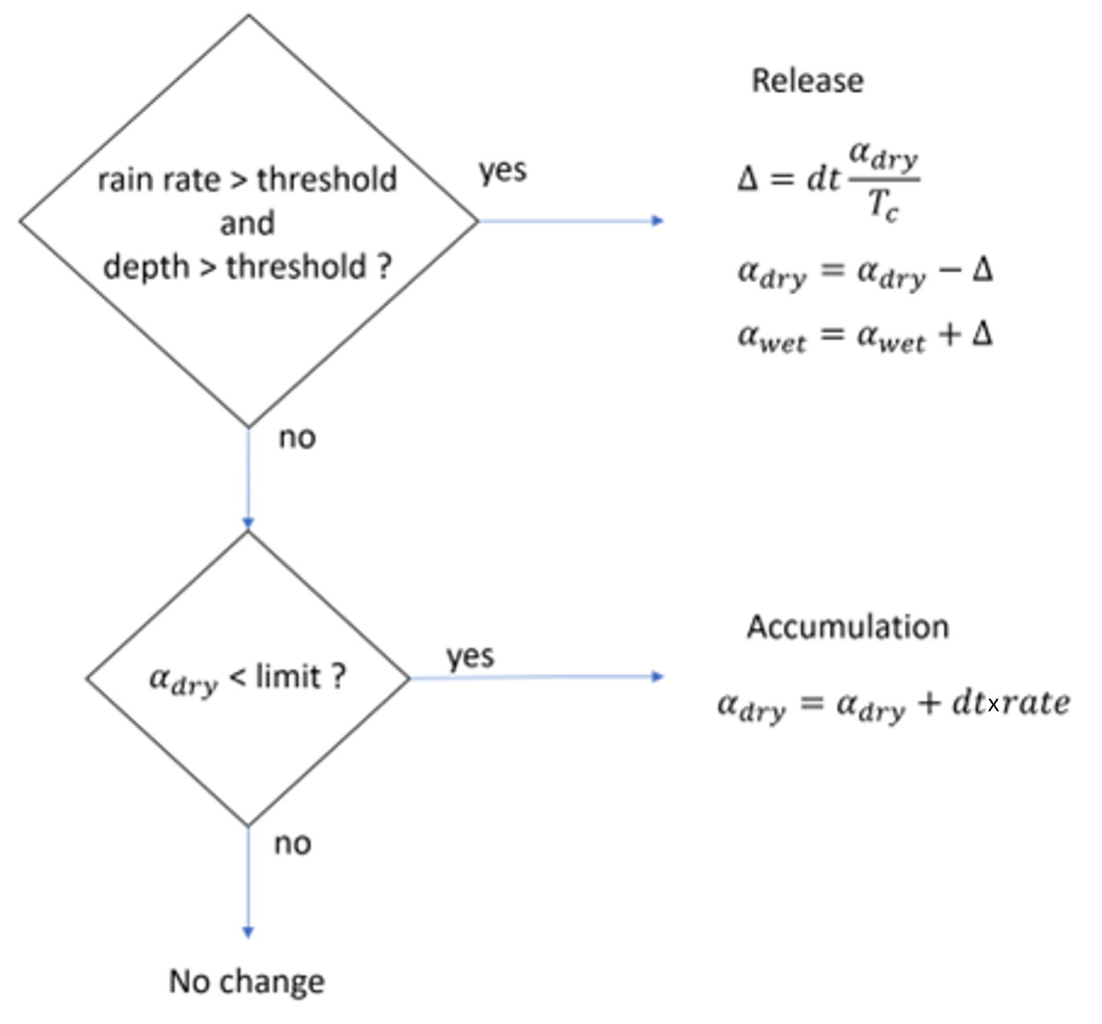
Figure 3.4: Washoff method

If a pollutant is released into its wet store, it is transported according to the progression of hydrologic and hydraulic flows (and associated advection and dispersion), which is completed as a separate calculation step to the generation update.

Settling velocities are assigned to individual pollutants, and may vary spatially with material. An example of where the latter might be applied is when sediment is known to flocculate in saline conditions and hence have its settling properties modified. Any settling returns pollutants from the wet store to the dry store. This is not recommended for dissolved pollutants, and where settling is to be turned off, the velocity should be set to zero. The mass flux per unit area in time \(dT\) due to settling \(\Delta\) (kg/ha) is given by Equation (3.2):

\[\begin{equation} \Delta = dT \times w_sC \tag{3.2} \end{equation}\]

w\(_s\) is the user specified settling velocity, \(C\) is the wet store cell concentration of pollutant. No other constraints to settling occurring are applied in this model.

If soils and subsurface flow (interflow) is not simulated in TUFLOW HPC, then this transport is purely surficial. If soils are included then released pollutants will be transported in both the surface and subsurface in accordance with water flows. TUFLOW CATCH allows for the optional prevention of infiltration of a given pollutant into the subsurface flow if soils are included in the TUFLOW HPC simulation. This is most relevant for particulate pollutants such as sediment or particulate organic material.

A conceptualisation of TUFLOW CATCH’s pollutant generation and transport methods is presented in Figure 3.5.

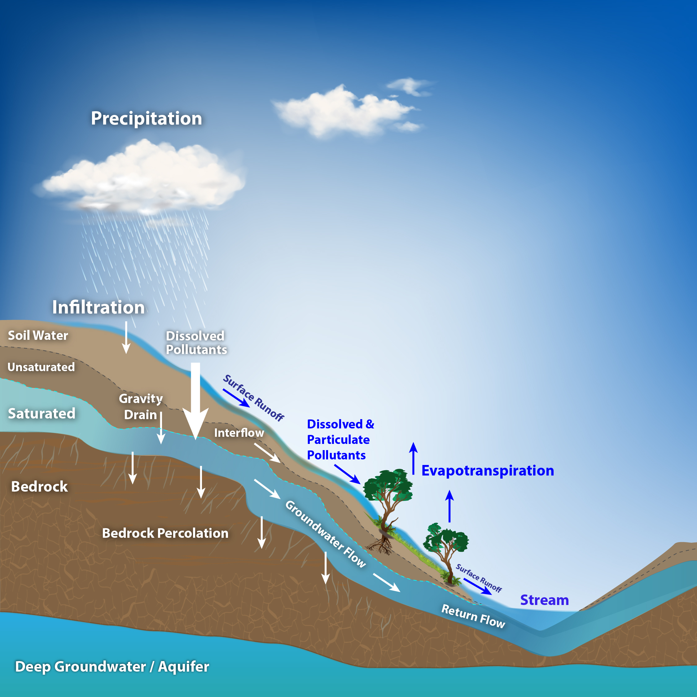
Figure 3.5: TUFLOW CATCH pollutant generation method

The relevant TUFLOW CATCH commands are described in Section 4.5.3.3.1.

3.2.3.2 Shear stress

Shear stress generation methods are common in natural waterway modelling studies (e.g. estuaries and coastal oceans), particularly with regard to the simulation of sediment transport. In short, these methods conceptualise sediment release from the bed as a function of overlying hydrodynamic shear stress: once a specified minimum shear stress is exceeded, sediment is released to the water column. Similarly, these methods also allow for deposition of previously suspended sediment back to the bed, and this is typically allowed to occur (at a set settling velocity) once ambient hydrodynamic shear stress drops below a specified maximum depositional shear stress. More advanced methods allow for construction of intermediary bed roughness models that translate raw hydrodynamic shear stress to the corresponding shear stress that is actually felt by the bed and can therefore cause erosion (or allow deposition). These methods therefore allow for the ongoing erosion and deposition of particulate materials as hydrodynamic conditions evolve in time and space. TUFLOW CATCH’s implementation of this method is described following. It is intended to be applied primarily to particulate pollutants, rather than dissolved.

3.2.3.2.1 Erosion

TUFLOW CATCH allows for the specification of erosion behaviour of any pollutant, on a spatially varying (material by material) basis. Even though this behaviour is specified per material, it is used to undertake erosion calculations on a cell by cell basis at the beginning of every timestep. For example, if a user has specified a 5 metre TUFLOW HPC grid size, then erosion calculations will be undertaken at this same spatial resolution. As each pollutant erodes from its dry store mass, it is released to its wet store and advected/dispersed accordingly. This removal is tracked and reported at the end of a simulation as a loss to each cell’s dry store mass (kg/ha).

TUFLOW CATCH adopts the Mehta erosion model on a cell by cell basis, such that the erosive flux \(\Delta\) (kg/ha) is given by Equation (3.3) in time \(dT\) (with appropriate units conversions):

\[\begin{equation} \Delta = dT \times E_r\left(\frac{\tau}{\tau_{ce}}-1\right)^{\alpha} \tag{3.3} \end{equation}\]

\(E_r\) is the erosion rate (g/m\(^2\)/s), \(\tau\) is the simulated hydrodynamic shear stress (N/m\(^2\)), \(\tau_{ce}\) is the user specified critical shear stress for erosion (N/m\(^2\)), \(\alpha\) is a dimensionless parameter set to 1.0 and \(\tau > \tau_{ce}\). TUFLOW CATCH does not deploy a bed roughness model so \(\tau\) is the pure hydrodynamic shear stress calculated from cell velocity. Once computed, eroded mass is tracked so that at simulation end, TUFLOW CATCH produces a map of eroded areas that allows for identification, for example, of ‘hotspot’ erosion locations. Users specify a limit to the mass of pollutant per unit area that is erodable within each material. This can be converted by the user to a depth via independent post processing steps if desired, by assuming a bulk density. This same output layer presents areas of accumulation, if this has occurred.

The relevant TUFLOW CATCH commands are described in Section 4.5.3.3.2.

3.2.3.2.2 Deposition

TUFLOW CATCH allows for the specification of depositional behaviour of any pollutant, on a spatially varying (material by material) basis. Even though this behaviour is specified per material, it is used to undertake deposition calculations on a cell by cell basis at the beginning of every timestep. As each pollutant deposits from its wet store mass, it is transferred to its dry store mass. This deposition is tracked and reported at the end of a simulation as a gain to each cell’s dry store mass (kg/ha).

TUFLOW CATCH adopts the Krone deposition model on a cell by cell basis within this pollutant export model, such that the areal depositional flux \(\Delta\) (kg/ha) in time \(dT\) is given by Equation (3.4). This is a more advanced version of the deposition approach used in the accumulation washoff model (Equation (3.2)).

\[\begin{equation} \Delta = dT \times \left(1-\frac{\tau}{\tau_{cd}}\right)w_sC \tag{3.4} \end{equation}\]

\(\tau\) is the raw hydrodynamic shear stress (N/m\(^2\)), \(\tau_{cd}\) is the user specified critical shear stress for deposition (N/m\(^2\)), w\(_s\) is the user specified settling velocity, \(C\) is the wet store cell concentration of pollutant and \(\tau < \tau_{cd}\).

The relevant TUFLOW CATCH commands are described in Section 4.5.3.3.2.