Appendix D Demonstration model
D.1 Context
A demonstration model and small suite of simulations have been developed to support TUFLOW CATCH users. These simulations:
- Can be used as templates for construction of other TUFLOW CATCH simulations
- Encompass the supported TUFLOW CATCH configurations, and
- Are able to be run without a licence for TUFLOW CATCH, TUFLOW HPC or TUFLOW FV
Descriptions of the model and demonstration simulations follow.
D.2 Domain
The demonstration model is located in New Zealand. It uses publicly available base data sets where available (with some of these being modified on occasion), and synthetic data otherwise.
The catchment has:
- An area of approximately 55km\(^2\)
- A relief of approximately 20m
- Three (synthetic) land uses
- Urban
- Forest
- Agriculture
The general arrangement of the catchment is presented in Figure D.1.
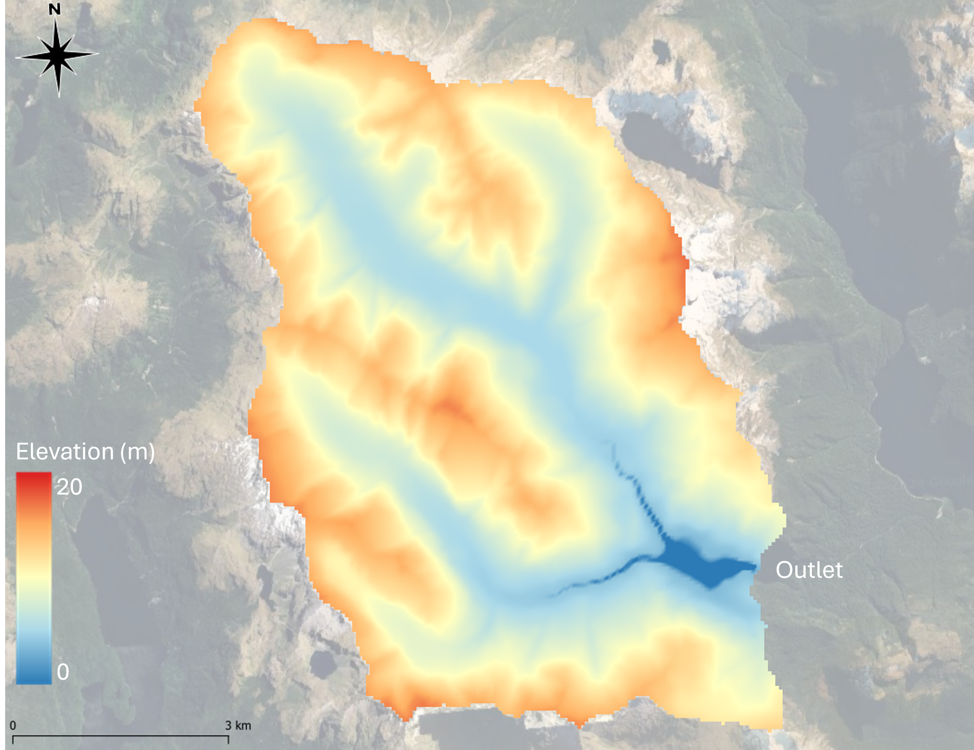
Figure D.1: TUFLOW CATCH demonstration model: catchment
The receiving waterway (which is a hypothetical lake) has:
- An area of approximately 1km\(^2\)
- A maximum depth of approximately 12m
- Two major riverine tributaries
- Two local wastewater treatment plant discharges
- One offtake
- An overflow outlet weir
The general arrangement of the receiving waterway is presented in Figure D.2.
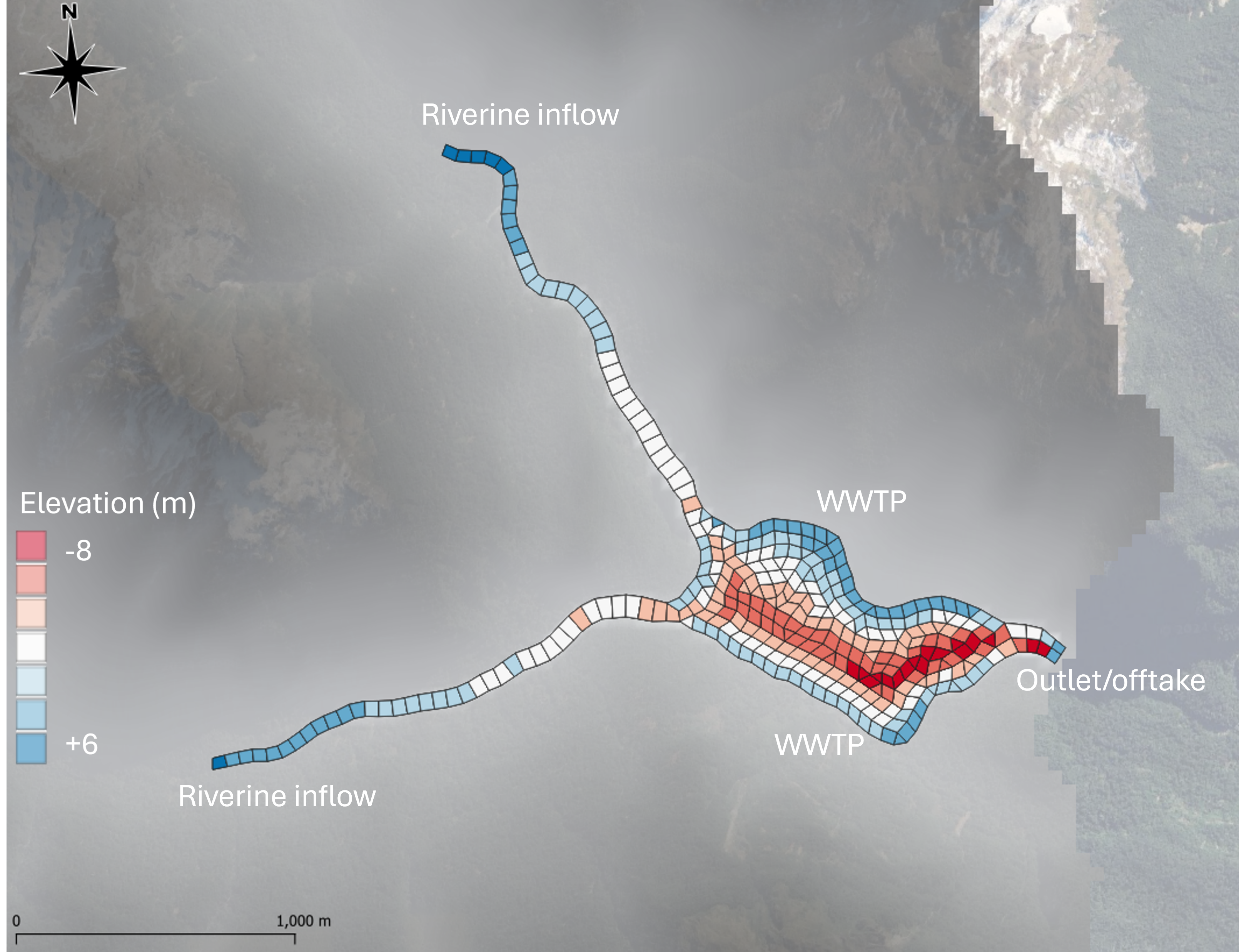
Figure D.2: TUFLOW CATCH demonstration model: receiving waterway
The domain is simulated under TUFLOW CATCH for a period of 1 week from 01/01/2021 to 07/01/2021, inclusive.
D.3 Numerical models
The TUFLOW HPC, pollutant export and TUFLOW FV models are described following.
D.3.1 TUFLOW HPC
The TUFLOW HPC model has the following general configuration:
- A 2D cell size of 50m, SGS turned on with a sample target distance of 1m
- A synthetic rainfall record applied, with a maximum daily rainfall of approximately 60mm
- Three materials, with one for each land use above
- One soil layer with constant thickness of 0.6m
All simulations use GPU.
D.3.2 Pollutant export
The pollutant export model has various forms depending on the TUFLOW CATCH configuration is simulated. Across these various forms, both Shear1 and Washoff1 methods are deployed, and other pollutant export parameters are set using the guidance provided in this manual. In all cases where applicable:
- Salinity, dissolved oxygen, silicate, adsorbed phosphorus and phytoplankton are set to constant concentrations
- Sediment and particulate organics are prohibited from infiltrating to groundwater
- Water temperature is provided as a timeseries
- Sediment uses the Shear1 method, and all other pollutants use the Washoff1 method
D.3.3 TUFLOW FV
The TUFLOW FV model has the following general configuration:
- Simulation of hydrodynamics, including density (salinity and temperature) driven processes
- Full atmospheric heat exchange simulation
- Sediment transport simulation, with one sediment fraction
- Water quality simulation, using the Organics simulation class
- 3D simulation with 8 z layers and 6 sigma layers
- Three bed materials to define sediment transport and water quality processes
All simulations use GPU.
D.4 Simulation suite
The demonstration model suite includes the following simulations.
| Simulation name | Description | Use case | TUFLOW CATCH Configuration |
|---|---|---|---|
| Demonstration_001.tcc | Catchment hydraulic calibration: HPC 2d outlet | Calibration of catchment hydraulic model without receiving model | TUFLOW HPC calibration only |
| Demonstration_002.tcc | Catchment hydraulic calibration: Pollutant export configuration with constant salinity and temperature timeseries | Calibration of catchment hydraulic model with downstream polygon | Pollutant export |
| Demonstration_003.tcc | Catchment pollutant calibration: Pollutant export configuration with user pollutant/s | Only catchment hydraulic and pollutant export models are to be used, with non-TUFLOW FV pollutants and downstream polygon | Pollutant export |
| Demonstration_004.tcc | Catchment pollutant calibration: Pollutant export configuration with TUFLOW FV pollutants | Calibration of catchment pollutant export model following 002 calibration, to TUFLOW FV pollutants with downstream polygon | Pollutant export |
| Demonstration_005.tcc | Linked catchment and receiving model: Integrated configuration with all TUFLOW FV pollutants | Generation of first pass spatially resolved TUFLOW FV HD and pollutant boundaries for subsequent TUFLOW FV calibration initiation | Integrated |
| Demonstration_006.tcc | Receiving model calibration: TUFLOW FV simulation with preserved inflows | Catchment hydraulic and pollutant modelling complete (or largely so) and TUFLOW FV is to be calibrated without reunning catchment model | Integrated |
| Demonstration_007.tcc | Linked catchment and receiving model: Hydrology configuration with salinity and temperature | No pollutant simulation required in TUFLOW - extend 002 above to include TUFLOW FV model | Hydrology |
D.5 Downloads
D.5.1 Binaries
The required binary executable files are to be downloaded from the following locations (to be updated with hyperlinks: in the interim, email support@tuflow.com for relevant binaries):
- TUFLOW CATCH
- TUFLOW HPC
- TUFLOW FV
It is suggested that these are saved in a convenient and centralised location. For the purposes of explanation in this Appendix, it has been assumed that they are saved to the following locations (with
C:\TUFLOW\EXE\TUFLOWCATCH\ReleaseXX\TUFLOWCATCH.exe C:\TUFLOW\EXE\TUFLOW\ReleaseYY\TUFLOW_iSP_w64.exe C:\TUFLOW\EXE\TUFLOWFV\ReleaseZZ\TUFLOWFV.exe
D.5.2 Simulation files
The demonstration model suite can be downloaded here, in the TUFLOW CATCH section. For the purposes of explanation in this Appendix, it has been assumed that the suite is saved to the following location and then unzipped:
C:\TUFLOW\Demonstration\TUFLOWCATCH\
When unzipped, the high level folder structure will be as follows:
- Modelling
- TUFLOW
- TUFLOWCATCH
- TUFLOWFV
The key directory for executing TUFLOW CATCH is then
C:\TUFLOW\Demonstration\TUFLOWCATCH\Modelling\TUFLOWCATCH\runs
Once downloaded and unzipped, the user is required to:
- In the
Modelling\TUFLOWCATCH\runs\run_simulation.bat file:On line 2, copy and paste in the exact path to the TUFLOW CATCH executable over the placeholder
<TUFLOW CATCH EXECUTABLE FULL PATH> , so that:
set exe = <TUFLOW CATCH EXECUTABLE FULL PATH>
becomes (using the example path above):
set exe = C:\TUFLOW\EXE\TUFLOWCATCH\ReleaseXX\TUFLOWCATCH.exe Uncomment the desired simulation command by deleting the preceding ‘
:: ’ , so that (if simulation 001 was to be run):
:: %exe% Demonstration_001.tcc
becomes:
%exe% Demonstration_001.tcc
- In the
Modelling\TUFLOWCATCH\runs\Demonstration_001.tcc file (and any other Demonstration_00*.tcc file to be executed):In the
CATCHMENT HYDRAULICS block, copy and paste in the exact path to the TUFLOW HPC executable over the placeholder<TUFLOW EXECUTABLE FULL PATH> , so that:
EXE == <TUFLOW EXECUTABLE FULL PATH>
becomes (using the example path above):
EXE == C:\TUFLOW\EXE\TUFLOW\ReleaseYY\TUFLOW_iSP_w64.exe In the
RECEIVING HYDRODYNAMICS AND WQ block, copy and paste in the exact path to the TUFLOW FV executable over the placeholder<TUFLOW FV EXECUTABLE FULL PATH> , so that:
EXE == <TUFLOW FV EXECUTABLE FULL PATH>
becomes (using the example path above):
EXE == C:\TUFLOW\EXE\TUFLOWFV\ReleaseZZ\TUFLOWFV.exe
Some text editors offer support for changing the above executable paths in multiple files at once, if required.
D.6 Execution
Once the binaries and simulation files have been downloaded and paths altered as above (and altered files saved), a TUFLOW CATCH simulation can be executed as follows:
- Open a command prompt and navigate to the TUFLOW CATCH runs folder:
- Ensure the path to the TUFLOW CATCH executable has been set in run_simulations.bat, and that at least one simulation has been uncommented
- Type the following in the command prompt and hit enter, and TUFLOW CATCH will execute:
Some notes on executing the demonstration simulations:
- Although not mandatory, it is suggested that the simulations be run one at a time, and in order, and results reviewed after each execution
- Demonstration_005.tcc must be run prior to Demonstration_006.tcc because the former generates boundary conditions for the latter.
- To ensure that Demonstration_006.tcc can access these boundaries generated by Demonstration_005.tcc, either:
- Manually make a copy of Demonstration_005_catchment_hydraulic.fvcatchbc and rename it as Demonstration_006_catchment_hydraulic.fvcatchbc in the same location, or
- Uncomment the line beginning ‘
copy… ’ in the run_simulations.bat file provided with the demonstration model (third line below)
D.7 Results interrogation
Once executed, results will be written to:
C:\TUFLOW\Demonstration\TUFLOWCATCH\Modelling\TUFLOWCATCH\results
Use the QGIS TUFLOW CATCH plugin (see Section 4.3) to generate a .json file and view the results. Simulations that involve only TUFLOW HPC or TUFLOW FV can have their *.xmdf and *.nc results interrogated in the normal manner through the TUFLOW Viewer as shown in Figure D.3.
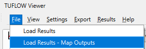
Figure D.3: TUFLOW CATCH demonstration model: loading standard TUFLOW HPC or TUFLOW FV results
D.7.1 Example json file creation
Simulations 005 and 006 can be used (after execution) to create a json file within the TUFLOW CATCH plugin (see Section 4.3). To do so, select the following results files in the json creation process (making sure the order in the selection dialogue box is as below):
- Demonstration_006_receiving_HD.nc
- Demonstration_006_receiving_WQ.nc
- Demonstration_005_catchment_hydraulic.xmdf
Save the json to here:
- C:\TUFLOW\Demonstration\TUFLOWCATCH\Modelling\TUFLOWCATCH\results\Demonstration_006.tuflow.json
Once created, drag and drop the json onto a QGIS window to view the results. Hit F7 to toggle the layer styling panel and reveal the full suite of simulated quantities. AS an example, select the ‘Conc SED_FINES’ field by clicking on the contour icon to the right of the field name as per Figure D.4.
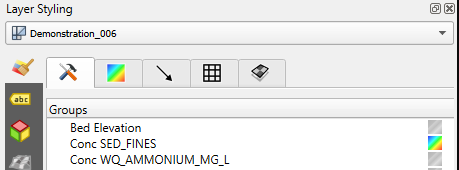
Figure D.4: Selecting the Conc SED-FINES data field in a json results file
An animation of the associated surface concentration results (that shows the connectivity between TUFLOW HPC, pollutant export and TUFLOW FV simulations of sediment) is presented in Figure D.5. This animation was prepared using the TUFLOW CATCH plugin, and the maximum concentration was set to 5 mg/L.

Figure D.5: Conc SEDFINES animated results
The connectivity between models is clear. Of note is the increase in concentrations once flows enter the receiving model arms. This is due to resuspension of previously accumulated bed sediment in the lake, which has been computed using the advanced TUFLOW FV Sediment Transport Module capability. Users could investigate this further by altering the erosion parameterisation within the TUFLOW FV sediment transport control file, or setting initial bed masses in the TUFLOW FV model to zero - this concentration spike will then not appear.
D.7.2 Example results
An example of a dry mass accumulation predicted by TUFLOW HPC (under the Washoff1 model) at a point in time just prior to rainfall is presented in Figure D.6, for FRP. The different accumulations of FRP in different land use areas are clear. The red areas are urban areas, which had the highest accumulation rates of FRP set within the simulation.
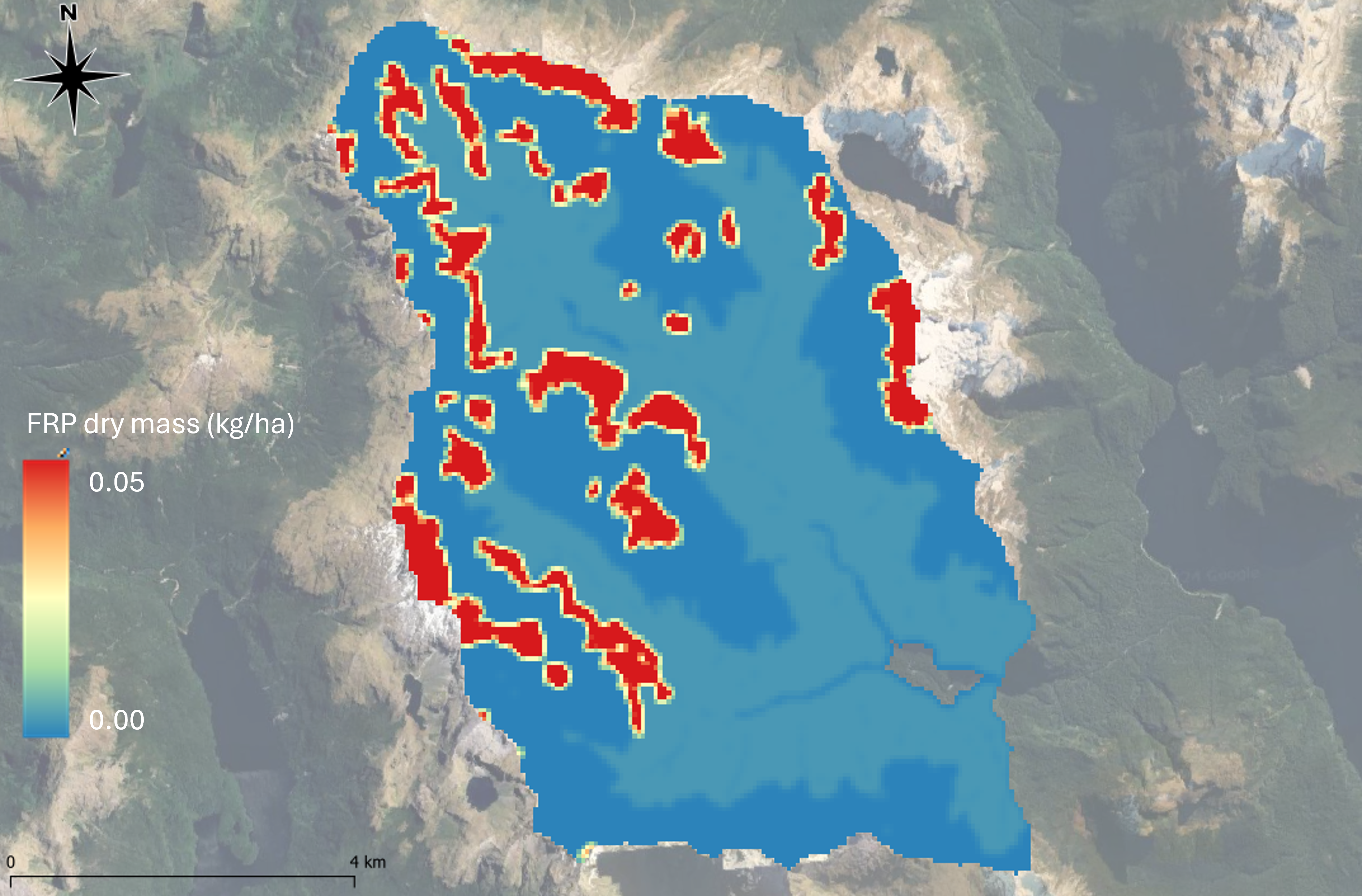
Figure D.6: TUFLOW CATCH demonstration model: FRP dry mass accumulation
An example of a net mass distribution predicted by TUFLOW HPC (under the Shear1 model) at simulation end is presented in Figure D.7, for SED_FINES. Positive (negative) results reflect net accumulation (erosion) at simulation end. Erosion (and deposition) limits were set to 1 kg/ha in the simulation. The figure shows that (at least) the catchment areas within the stream network have been eroded to this maximum (blue colour), and no more.
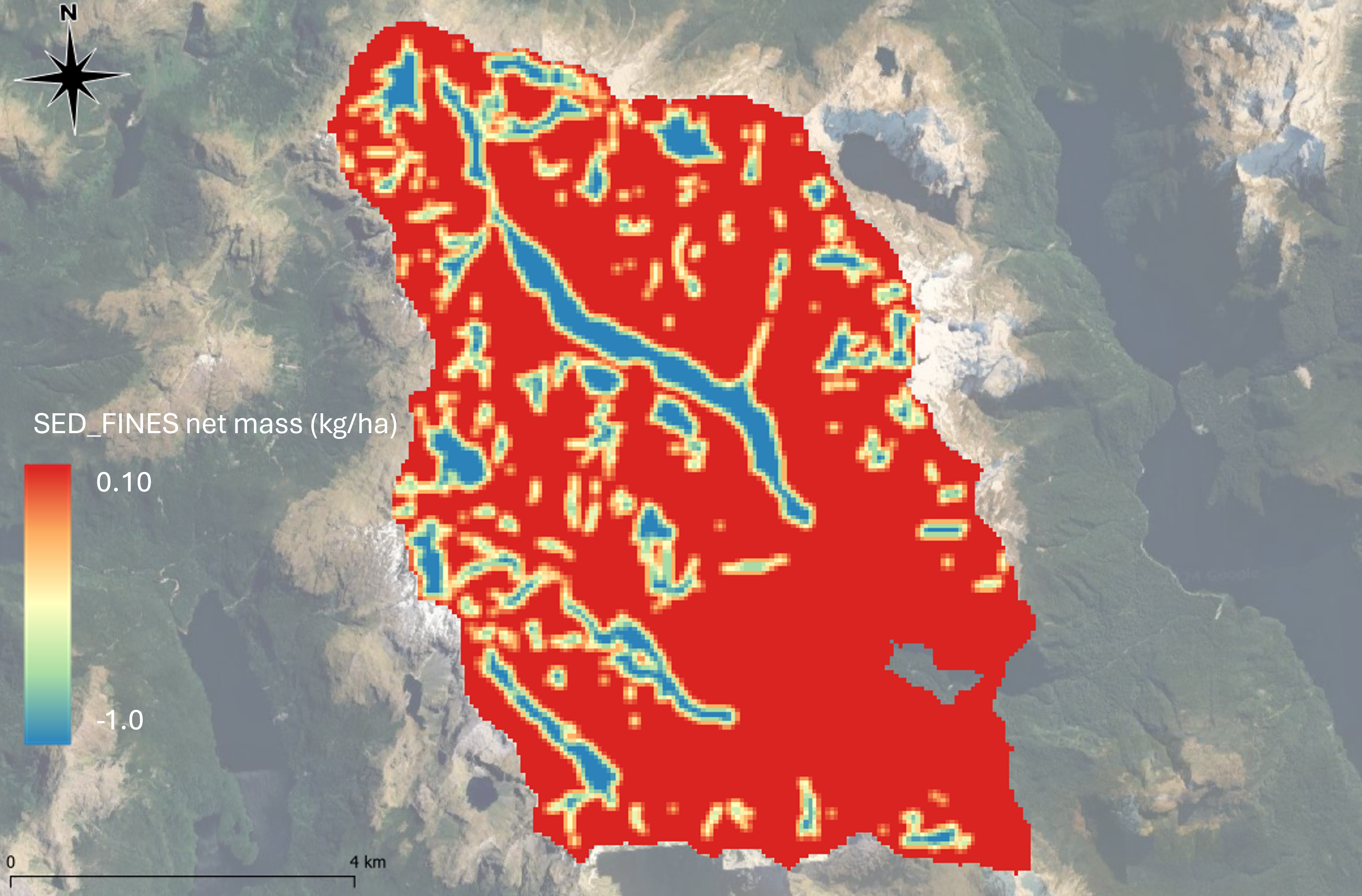
Figure D.7: TUFLOW CATCH demonstration model: SEDFINES net mass at simulation end
