D.7 Results interrogation
Once executed, results will be written to:
C:\TUFLOW\Demonstration\TUFLOWCATCH\Modelling\TUFLOWCATCH\results
Use the QGIS TUFLOW CATCH plugin (see Section 4.3) to generate a .json file and view the results. Simulations that involve only TUFLOW HPC or TUFLOW FV can have their *.xmdf and *.nc results interrogated in the normal manner through the TUFLOW Viewer as shown in Figure D.3.
Figure D.3: TUFLOW CATCH demonstration model: loading standard TUFLOW HPC or TUFLOW FV results
D.7.1 Example json file creation
Simulations 005 and 006 can be used (after execution) to create a json file within the TUFLOW CATCH plugin (see Section 4.3). To do so, select the following results files in the json creation process (making sure the order in the selection dialogue box is as below):
- Demonstration_006_receiving_HD.nc
- Demonstration_006_receiving_WQ.nc
- Demonstration_005_catchment_hydraulic.xmdf
Save the json to here:
- C:\TUFLOW\Demonstration\TUFLOWCATCH\Modelling\TUFLOWCATCH\results\Demonstration_006.tuflow.json
Once created, drag and drop the json onto a QGIS window to view the results. Hit F7 to toggle the layer styling panel and reveal the full suite of simulated quantities. AS an example, select the ‘Conc SED_FINES’ field by clicking on the contour icon to the right of the field name as per Figure D.4.
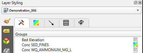
Figure D.4: Selecting the Conc SED-FINES data field in a json results file
An animation of the associated surface concentration results (that shows the connectivity between TUFLOW HPC, pollutant export and TUFLOW FV simulations of sediment) is presented in Figure D.5. This animation was prepared using the TUFLOW CATCH plugin, and the maximum concentration was set to 5 mg/L.

Figure D.5: Conc SEDFINES animated results
The connectivity between models is clear. Of note is the increase in concentrations once flows enter the receiving model arms. This is due to resuspension of previously accumulated bed sediment in the lake, which has been computed using the advanced TUFLOW FV Sediment Transport Module capability. Users could investigate this further by altering the erosion parameterisation within the TUFLOW FV sediment transport control file, or setting initial bed masses in the TUFLOW FV model to zero - this concentration spike will then not appear.
D.7.2 Example results
An example of a dry mass accumulation predicted by TUFLOW HPC (under the Washoff1 model) at a point in time just prior to rainfall is presented in Figure D.6, for FRP. The different accumulations of FRP in different land use areas are clear. The red areas are urban areas, which had the highest accumulation rates of FRP set within the simulation.

Figure D.6: TUFLOW CATCH demonstration model: FRP dry mass accumulation
An example of a net mass distribution predicted by TUFLOW HPC (under the Shear1 model) at simulation end is presented in Figure D.7, for SED_FINES. Positive (negative) results reflect net accumulation (erosion) at simulation end. Erosion (and deposition) limits were set to 1 kg/ha in the simulation. The figure shows that (at least) the catchment areas within the stream network have been eroded to this maximum (blue colour), and no more.
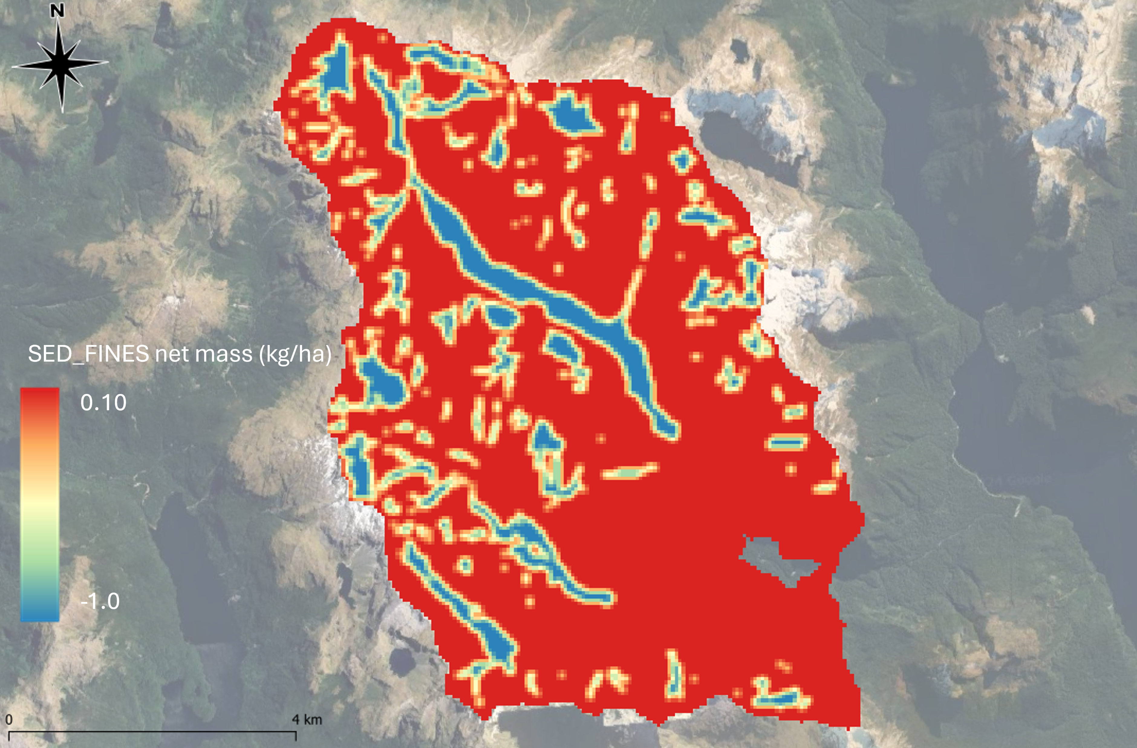
Figure D.7: TUFLOW CATCH demonstration model: SEDFINES net mass at simulation end