Appendix B Vertical Mixing Model Benchmarking

B.1 Overview

This section presents the results from three foundational benchmark tests that increase in complexity. Results are compared with theoretical solutions where appropriate. The tests are:

1. Open channel turbulent flow
2. Wind induced circulation in a lake
3. Deepening of a wind-mixed layer

The first two tests focus on unstratified flow without the impact of Earth’s rotation, whilst the third test is conducted in stably stratified field, both with and without the action of Coriolis forcing.

B.2 Open Channel Flow

An open channel flow represents one of the most fundamental turbulent flow scenarios. In this test, an unstratified flow in a 1000 m long, 50 m wide, and 5 m deep rectangular channel with a uniformly rough surface (Manning’s n = 0.03) was investigated. The bed slope was set at 0.00042 to achieve a uniform flow with a depth-averaged velocity of 2 m/s. The horizontal mesh size was 10 m by 10 m, while the vertical mesh size used in the simulations was 0.25 m (Figure B.1).

Figure B.1: Model Mesh - Open Channel Flow Benchmark

The vertical profile of the velocity follows the Law of the Wall, and the vertical profile of the eddy viscosity \(\nu_t\) is expressed by a parabolic function:

\[ \nu_t = \kappa h u_* \frac{z}{h} \left(1 - \frac{z}{h} \right) \]

Where:

• \(\kappa\) is the von Karman constant (0.41)
  
• \(h\) is the water depth (m)
  
• \(z\) is the vertical coordinate (m)
  
• \(u_*\) is the bed shear velocity (m/s), calculated as:

\[ u_* = \left( g^{1/2} n \right) h^{-1/6} \bar{U} \]

Where:

• \(\bar{U}\) is the depth-averaged velocity (\(m/s\))
• \(g\) is the gravitational acceleration (\(m/s^2\))
• \(n\) is the Manning’s ‘n’ roughness (\(s/m^{1/3}\))

Figure B.2 presents the vertical profiles of the horizontal velocity and \(\nu_t\) modelled using the k-ε and k-ω turbulence models with default parameters. The solutions of the two models are similar and agree well with the empirical solutions. The k-ω model predicts a higher maximum eddy viscosity at half-depth compared with the k-ε model.

Figure B.2: Vertical profiles of horizontal velocity (left) and eddy viscosity (right) in a straight open channel simulated by k-ε and k-ω models

B.3 Wind Circulation

The wind circulation test represents an unstratified flow in a 1000 m long, 10 m deep, flat-bottomed rectangular lake. The flow is driven by a constant surface wind stress in the x-direction. Momentum is entrained into the deeper layer due to shear stress between vertical layers. A bottom current forms in the opposite direction to the wind forcing in accordance with mass conservation.

The horizontal mesh size was 10 m in the wind direction, with a single cell across the width of the lake. The vertical mesh thickness was set to 0.5 m (Figure B.3). Bed roughness effects were assumed negligible, with a roughness length scale \(k_s = 0.05\).

Figure B.3: Model Mesh - Wind Circulation Benchmark

The analytical solution for the vertical velocity profile is:

\[ U(z) = \frac{u_s}{\kappa} \left[1 + \ln\left(\frac{h - z}{h}\right)\right] \]

Where the surface shear velocity \(u_s\) is given by:

\[ u_s = \left( \frac{\tau_s}{\rho_w} \right)^{1/2} \]

And the surface shear stress \(\tau_s\) is calculated from:

\[ \tau_s = \rho_a C_d W_{10}^2 \]

Where:

• \(u_s\) is the surface shear velocity (m/s)
  
• \(\tau_s\) is the surface shear stress (N/m²)
  
• \(\rho_w\) is the water density (= 1000 kg/m³)
  
• \(\rho_a\) is the air density (= 1.2 kg/m³)
  
• \(C_d\) is the wind drag coefficient (0.0013)
  
• \(W_{10}\) is the wind speed 10 m above the surface (assumed 20 m/s in this test)

Assuming the vertical profile of the eddy viscosity also follows a parabolic function, the bed shear velocity can be replaced by the surface shear velocity \(u_s\) in the parabolic function below:

\[ \nu_t = \kappa h u_s \frac{z}{h} \left(1 - \frac{z}{h}\right) \]

Figure B.4 presents the vertical profiles of horizontal velocity and \(\nu_t\) modelled using the k-ε and k-ω turbulence models with default parameters. The results from both models agree well with empirical solutions, with the k-ω model showing nearly perfect agreement for velocity.

Figure B.4: Vertical profiles of velocity (left) and eddy viscosity (right) driven by constant wind over a rectangular lake, simulated using k-ε and k-ω turbulence models

B.4 Entrainment Of Wind Mixed Layer

The previous two tests examined unstratified flow at equilibrium. This test simulates the dynamic entrainment and deepening of a wind-driven surface mixed layer in stably stratified flow. Entrainment is driven by surface wind stress, gradually eroding the stratified fluid below.

Pollard et al. (1973) proposed a simple model for the deepening of the surface mixed layer. In the absence of the Coriolis force, the evolution of the mixed-layer depth \(h_{\text{MLD}}\) is given by:

\[ h_{\text{MLD}} = (2 R_{i,b})^{1/4} u_s \sqrt{\frac{t}{N_0}} \]

Where:

• \(R_{i,b}\) is the bulk Richardson number
  
• \(u_s\) is the surface shear velocity (m/s)
  
• \(t\) is the time since the onset of wind (s)
  
• \(N_0\) is the initial Brunt–Väisälä frequency (s\(^{-1}\))
  
• \(\rho_a\) is the air density (1.2 kg/m³)

The test model consisted of one horizontal cell, 50 m deep, with 50 vertical layers. Zero-gradient boundaries were applied on all sides. A constant surface shear stress of 0.1 N/m² was applied in the x-direction. An inverse water temperature profile was used to set an initial stratification of \(N_0 = 0.01 \,\text{s}^{-1}\).

Figure B.5: Model Mesh - Wind Entrainment Benchmark

Figure B.6 and Figure B.7 show the development of the surface mixed-layer following wind onset, modelled with the k-ε and k-ω turbulence models, respectively. Dashed lines represent the empirical prediction by Pollard et al. (1973), using \(R_{i,b} = 0.6\) as suggested by Price (1979). Both turbulence models in TUFLOW FV reproduce the deepening of the surface mixed layer effectively.

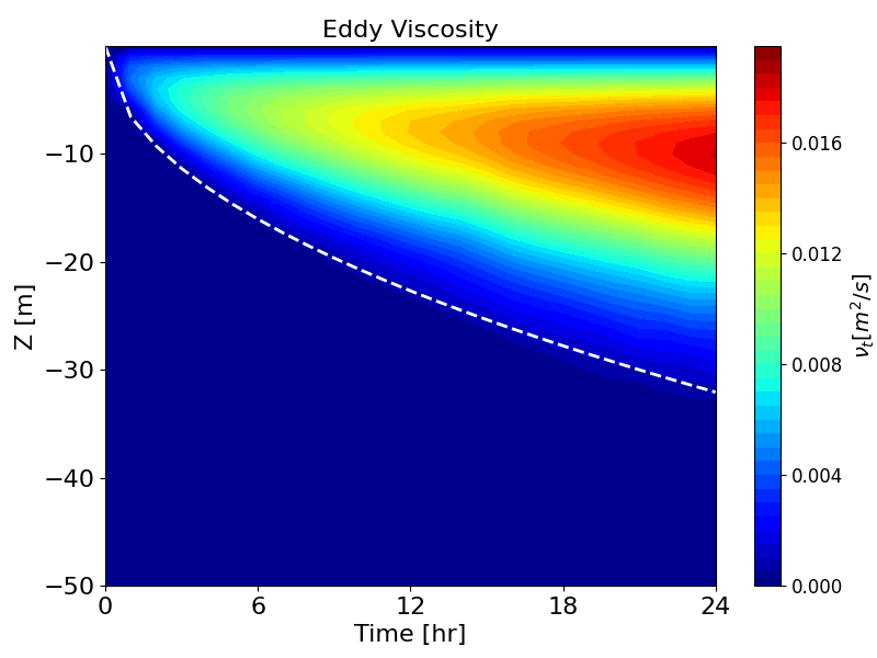
Figure B.6: Hovmöller diagrams of velocity (left) and eddy viscosity (right) over time, simulated by k-ε model. Dashed lines show the empirical model by Pollard et al. (1973)

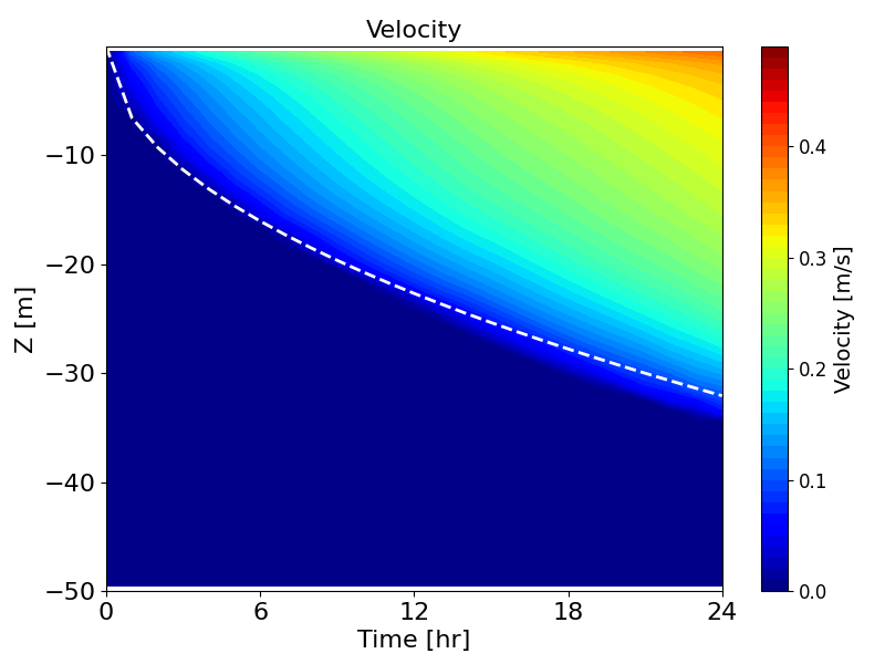
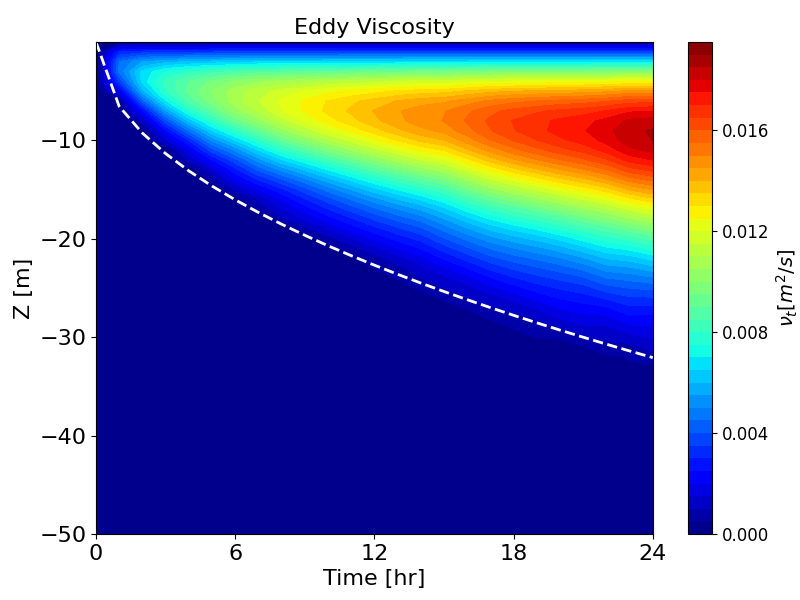
Figure B.7: Hovmöller diagrams of velocity (left) and eddy viscosity (right) over time, simulated by k-ω model. Dashed lines show the empirical model by Pollard et al. (1973)

Figure B.8 and Figure B.9 present the same wind entrainment test results, but with the second-order turbulence model (Umlauf and Burchard, 2005) enabled.

Compared to the results without second-order closure, the eddy viscosity is damped, and the surface mixed-layer develops slightly more slowly. This produces better agreement with the analytical solution of Pollard et al. (1973).

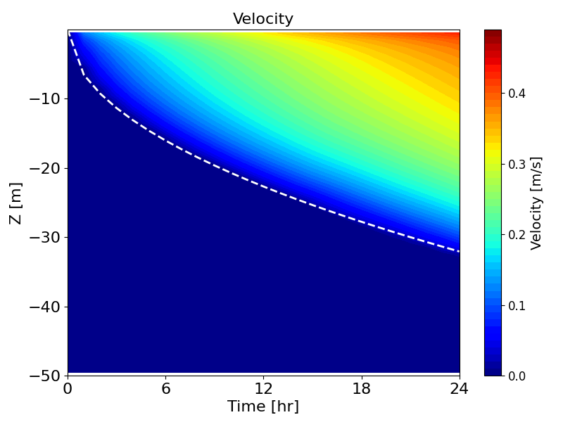
Figure B.8: Hovmöller diagrams of velocity (left) and eddy viscosity (right) over time, simulated by k-ε model with second-order turbulence model. Dashed lines show the empirical model by Pollard et al. (1973)

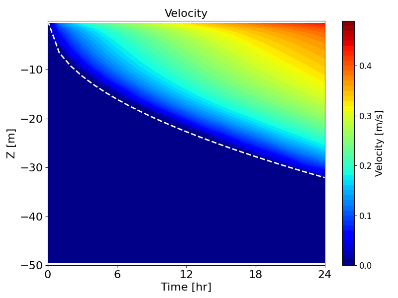
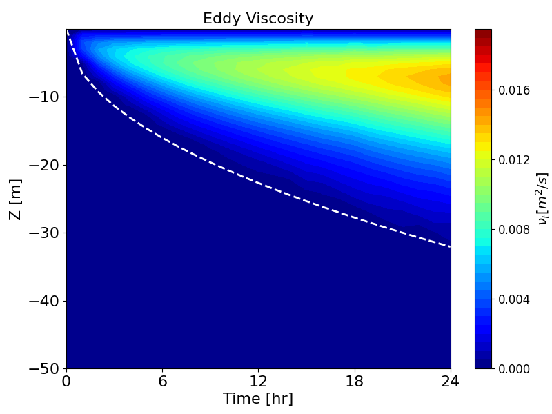
Figure B.9: Hovmöller diagrams of velocity (left) and eddy viscosity (right) over time, simulated by k-ω model with second-order turbulence model. Dashed lines show the empirical model by Pollard et al. (1973)

B.4.1 Wind Entrainment With Coriolis Forcing

The previous simulations were conducted without considering Earth’s rotation. This is valid for small systems (i.e., where characteristic length scales are smaller than the local Rossby radius). However, for larger systems, such as the open ocean away from the equator, the Coriolis force must be considered. It is known to generate features such as Ekman spirals (Figure B.10).

Figure B.10: Northern Hemisphere Ekman spiral illustrated by Cardin and Olson (2015)

When Ekman spirals form, the velocity oscillates with a characteristic period called the inertial period \(T_f\), which is defined by:

\[ T_f = \frac{2\pi}{f}, \quad f = 2\Omega \sin\phi \]

Where:

• \(f\) is the Coriolis parameter (s\(^{-1}\))
  \(\Omega = 7.2921 \times 10^{-5} \,\text{rad/s}\) (Earth’s angular speed)
• \(\phi\) is the latitude (degrees)

Pollard et al. (1973) suggest that the surface mixed layer deepens rapidly within the first \(0.5T_f\) after wind onset, and the rate of deepening decreases significantly thereafter as Ekman spirals form. The predicted mixed-layer depth at \(0.5T_f\) is given by:

\[ h_{\text{MLD}} = (8 R_{i,b})^{1/4} \frac{u_s}{\sqrt{N_0 f}} \]

An additional test was conducted at a latitude of 45° north, resulting in a Coriolis parameter of:

\[ f = 1.03 \times 10^{-4} \,\text{rad/s} \]

This corresponds to an inertial period of:

\[ T_f = \frac{2\pi}{f} = 16.97 \,\text{hours} \]

Figure B.11 and Figure B.12 present the development of velocities in the x-direction (aligned with the wind) and y-direction (perpendicular to the wind).

The velocity in the x-direction increased until approximately \(0.5T_f\), then decreased until \(T_f\). After this, the velocity exhibited periodic oscillations with the inertial period of 16.97 hours.

In the y-direction (toward the equator), a negative velocity developed, which also oscillated with the same period, consistent with the formation of an Ekman spiral.

As predicted by Pollard et al. (1973), the surface mixed-layer depth increased rapidly until \(0.5T_f\), and then continued to increase, but at a much slower rate. The modelled mixed-layer depth agrees well with the analytical prediction at \(0.5T_f\), shown as white dashed lines in the figures. The continued deepening beyond \(0.5T_f\) aligns with the results from Large Eddy Simulations (LES) performed by Ushijima and Yoshikawa (2020).

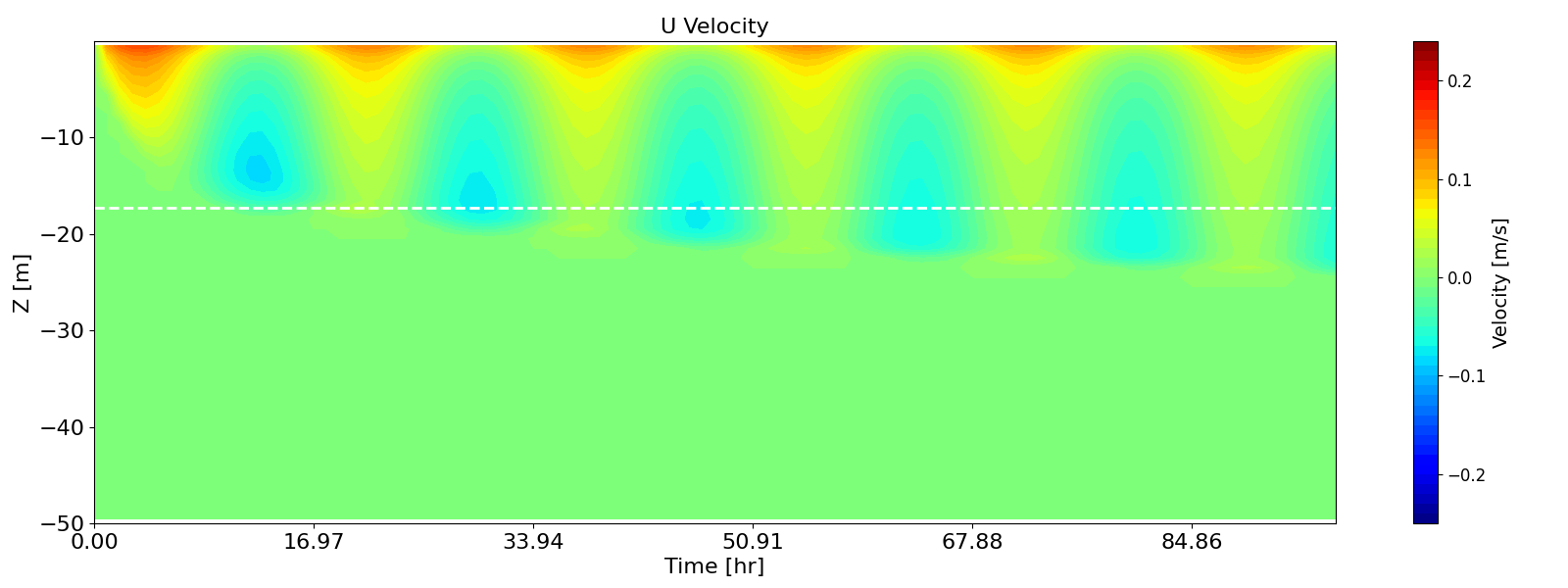
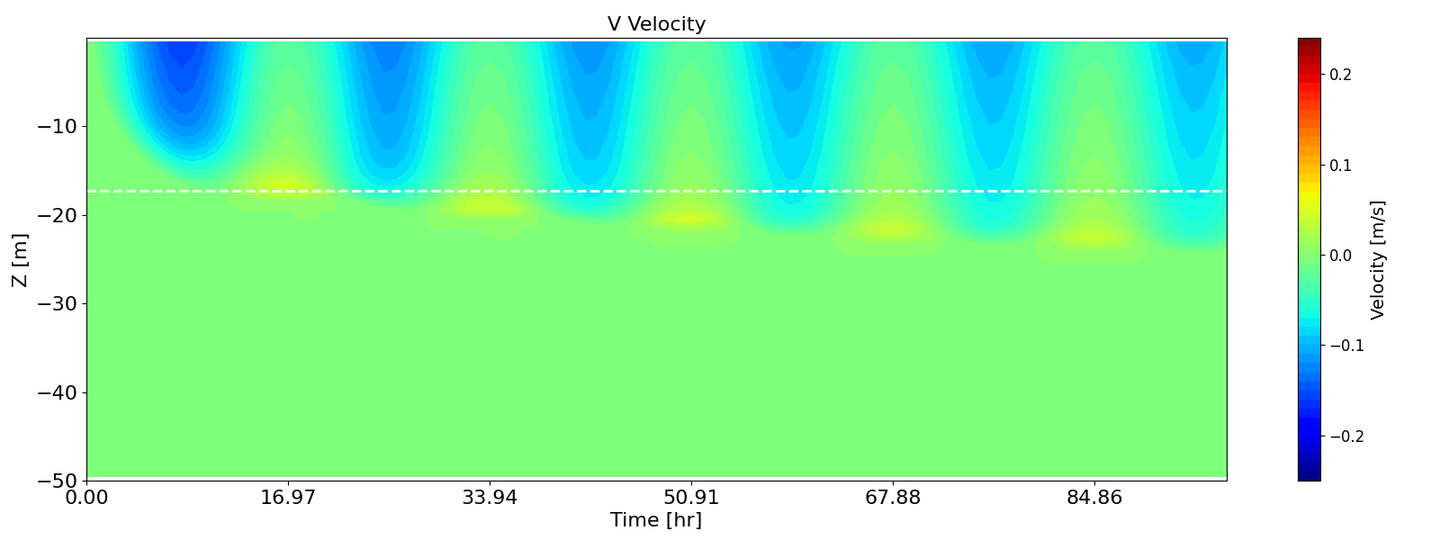
Figure B.11: Hovmöller diagrams of velocity in the x- (wind direction, top) and y- (perpendicular to the wind, bottom) directions, simulated by k-ε model with the second-order turbulence model enabled

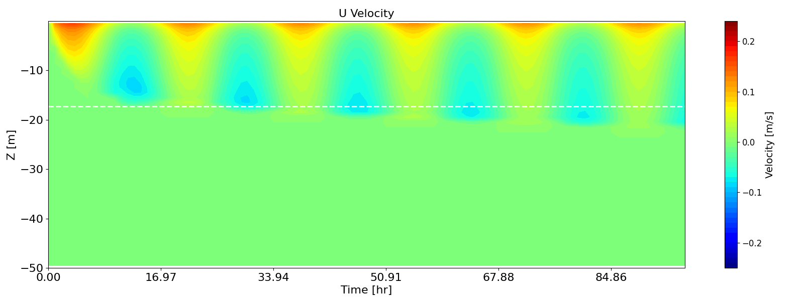
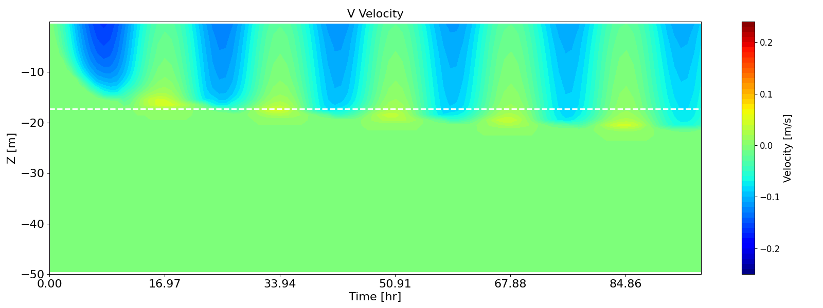
Figure B.12: Hovmöller diagrams of velocity in the x- (wind direction, top) and y- (perpendicular to the wind, bottom) directions, simulated by k-ω model with the second-order turbulence model enabled

B.5 References

References are provided in Section 3.6.