8.4 2D Boundaries (2d_bc, 2d_sa and 2d_rf Layers)

2D boundary conditions and linkages between the 1D and 2D domains are defined using a combination of one or more 2d_bc, 2d_sa or 2d_rf GIS layers. The different types of boundaries and links are described in Table 8.5.

Conditions have been built into TUFLOW to ensure a cell can only be assigned one boundary from a single GIS layer (except for: pit SX connections; sink/source points or lines with two vertices only; and polygon boundaries such as SA and RF).

Error checks have been incorporated into TUFLOW during the input pre-processing of 2D boundary conditions, TUFLOW stops with an error if a cell is:

• Assigned a HT or HS that is already a QT, SX, ST or HX cell;
  
• Assigned a 2D or HX that is already any other boundary;
• Assigned a QT that is already a SX or H boundary; and
  
• Assigned a ST or SX that is already a QT or H boundary.

Table 8.5: 2D Boundary Condition and Link Types

Type	Description	Comments
Water Level Boundaries
HQ	Water Level (Head) versus Flow (Q)	Assigns a water level to the cell(s) based on a water level versus flow (stage-discharge) curve. Alternatively, TUFLOW can automatically generate the HQ curve if a slope is specified using the 2d_bc GIS layer “b” attribute (see Table 8.6). The variation in Manning’s n with depth feature is taken into account if automatically calculating the stage-discharge curve.
HT	Water Level (Head) versus Time	Assigns a water level to the cell(s) based on a water level versus time curve. Uses the 2d_bc GIS layer (See Section 8.4.1).
HX	Water Level (Head) from an eXternal Source (i.e. a 1D model)	For linking 1D and 2D domains. One or two 1D nodes provide a water level to the 2D every half timestep. TUFLOW automatically creates 1D QX boundaries at the 1D node(s) (see Table 8.3), which also receives flow from the 2D domain every half timestep. 2D HX boundaries are linked to 1D nodes using CN connections (see below and Figure 10.4). Uses the 2d_bc GIS layer (See Section 8.4.1).
2D	Links two 2D domains	Multiple domain boundary only available for TUFLOW Classic. Refer to Section 10.7.2. Uses the 2d_bc GIS layer (See Section 8.4.1).
HS	Sinusoidal (Tidal) Water Level (m)	Legacy boundary condition, available for Classic solver only. HT boundary is the recommended alternative. Refer to the 2018 TUFLOW Manual for further details.
Treatment		Cell(s) can be wet or dry. It is not a requirement that at least one cell is wet. All H line types can be oblique to the X-Y axes. The water level can vary in height along a line of cells. Tip: A common cause of instabilities at or near head boundaries at the start of a simulation is the initial water level specified at the adjacent cells is different to the head value. If your model immediately goes unstable or requires a very low timestep at the boundary, check your initial water levels. If it is a 2D HX boundary, the water levels in the 1D node and the 2D cells should be similar.
Combinations		Multiple water level boundaries that select the same cell are not recommended. For TUFLOW Classic, multiple HT or HS boundaries can be applied and the water level used is the sum of the water levels assigned. This is not recommended, and is not supported in TUFLOW HPC.
Groundwater Boundaries
GT	Groundwater Level versus Time	Assigns a groundwater level to the cell(s) based on a groundwater level versus time curve. The same groundwater level boundary applies to all vertical soil layers. If the specified groundwater level is below the elevation at the bottom of the layer, it is dry. If the specified groundwater level is above the elevation at the top of the layer, it is fully saturated. Uses the 2d_bc GIS layer (See Section 8.4.1).
Flow Boundaries	(Directional)
QT	Flow versus Time (m3/s)	Distributes flow in quantity and direction across the cell(s) based on their topography, bed roughness and whether upstream or downstream controlled flow. The limiting assumption is that the water level along the line is constant, and the line must be digitised roughly perpendicular to the flow and should avoid areas where significant super-elevation or other similar effects occur. Cells can wet and dry, the line can be oblique to the grid. Multiple QT boundaries should not be applied to the same cell.
Flow Boundaries	(non-Directional)
RF	Rainfall versus Time (mm) Infiltration versus Time (mm)	Applies a rainfall hyetograph. The rainfall time-series data must be in mm depth per timestep. It is converted to a hydrograph to smooth the transition from one rainfall period to another (the converted hydrograph appears in the .tlf file for cross-checking). Note: the input curve is not mm/h versus timestep, but mm vs timestep (i.e. each rainfall value is the amount of rain that fell in mm between the previous time and the current time). Uses the 2d_rf GIS layer (see Section 8.4.3).
SA	Flow versus Time (m3/s) over an area, or Rainfall versus Time (mm)	Applies the flow directly onto the cells within the polygon as a source. Negative values remove water directly from the cell(s). Most commonly used to model rainfall-runoff directly onto 2D domains with each polygon representing the sub-catchment of a hydrology model. SA boundaries have their own command, Read GIS SA, and own GIS layer, 2d_sa. Uses the 2d_sa GIS layer (see Section 8.4.2).
SD SH	Flow versus Depth or Head (m3/s)	Extracts the flow directly from the cells based on the depth (SD) or water level (SH) of the cell. Used for modelling pumps or other water extraction. Flow values must not be negative. SD or SH boundaries can be connected to another 2D cell or a 1D node, to model the discharge of a pump from one location in a model to another. The connection is made using a “SC” line (see below). In the boundary condition database, the Column 1 data would be depth (SD) or water level (SH) values and the Column 2 data would be flow. The flow value is the rate per 2D cell. If the 2D cell becomes dry, no flow occurs. Uses the 2d_bc GIS layer (see Section 8.4.1). An example 2D pump model is available in the Example Model Dataset on the TUFLOW Wiki. This boundary is not supported when using Quadtree and ERROR 2815 will be reported.
ST	Flow versus Time (m3/s)	Applies the flow directly to the cells as a source. Negative values remove water directly from the cell(s). Can be used to model concentrated inflows, pumps, springs, evaporation, etc. The flow specified in the boundary file is applied to each cell to which the boundary is connected. For example, if the boundary file specifies 2 m3/s and the ST is applied over four cells, then the total flow applied to the model would be 8 m3/s. If the total flow required is 2 m3/s, then an f attribute of 0.25 could be applied so that only 0.5 m3/s is applied to each cell. Uses the 2d_bc GIS layer (see Section 8.4.1). Alternatively, the Read GIS SA ALL could be used to distribute a flow equally over a number of cells.
SX	Source of flow from a 1D model.	For linking 1D and 2D domains. 2D SX cell(s) are connected to a 1D node using a single CN connection (see below). The net flow into/out of the 1D node is applied as a source to the 2D cells. For example, a 1D pipe in the 2D domain “sucks” water out of the upstream cell(s) and “pours” water back out at the downstream cell(s) using 2D SX boundaries. Uses the 2d_bc GIS layer (see Section 8.4.1). If an SX cell falls on an inactive cell (Code -1 or 0), the cell is set as active (Code 1).
Treatment		Sources are applied to all the specified cell(s) whether they are wet or dry, except for SA and SX, which apply only to wet cells, or the lowest dry cell if all the SA or SX cells are dry. Uses the 2d_bc GIS layer (see Section 8.4.1).
Combinations		Any number of source boundaries can be assigned to the same cell(s) whether they are SA, SD, SH, ST or SX. The source rate applied is the sum of the individual sources.
Connections
CN	Connection of 2D HX and 2D SX boundaries to 1D nodes	Used in GIS 2d_bc layers (see Section 8.4.1) to connect 2D HX and 2D SX boundaries to 1D nodes. A line is digitised that snaps the 2D HX or SX object to the 1D node. The direction or digitised length of the line is not important. The 1D node would be in a 1d_nwk layer. Note that if the 2D SX object is snapped to the 1D node, no CN object is required. However, 2D HX objects always require a CN object to connect to the 1D node. Alternatively, a CN point object can also be used instead of a line. An ERROR occurs if a CN object is not snapped to a 2D HX or 2D SX object, or is redundant (i.e. not needed). For backward compatibility, use Unused HX and SX Connections (.tcf file) or Unused HX and SX Connections (.tbc file) to change the ERROR to a WARNING. Note that for connections to 2D SX objects only one (1) CN object is required. Whereas 2D HX objects must have a minimum of two (2) CN objects – one at each end – with intermediate CN objects as needed to connect to any 1D nodes. The same node can be connected to each end of a HX line if the water level should not vary along the line.
SC	Connection of 2D SD and SH boundaries	Used for connecting 2D SD and SH boundaries to another 2D cell or 1D node (e.g. modelling the pumping of water from one location to another). The direction of the line is important and should be digitised from the SH/SD pump towards the 2D cell or node which the water is to be transferred to. Uses the 2d_bc GIS layer (see Section 8.4.1). An example 2D pump model is available in the Example Model Dataset on the TUFLOW Wiki. This boundary is not supported when using Quadtree and ERROR 2815 will be reported.
Wind
WT	Modelling Wind Stresses as a force on the water column	Legacy boundary condition and not recommended for use. Suggest use of the cyclone/hurricane (See Section 8.6) or external stress boundary (See Section 8.7) instead. Refer to the 2018 TUFLOW Manual for details on WT boundary.
Variable Geometry
VG	Modelling of breaches, etc.	Supported in TUFLOW Classic only. Not supported in TUFLOW HPC (including Quadtree). Used for varying cell elevations over time. Each cell, or line of cells, needs to be assigned a time series of elevations in the same manner that other boundaries are applied. Also see Section 7.2.6.3 on Variable Z Shape layers as a simpler alternative. Note: If varying the elevations of a HX cell, the elevation must not fall below the 1D bed value (see the attributes of the 1d_to_2d_check file for that cell). No run-time checks are made in this regard. Also see VG Z Adjustment.
Other
CD	Code Polygon	Objects in a GIS 2d_bc layer (see Section 8.4.1) used to define the grid’s cell codes using Read GIS Code BC as an alternative to Read GIS Code. The code value is set using the f attribute (see Table 8.6). The boundary lines are snapped to “CD” regions so that if the boundary location is adjusted, the boundary line and code region can move together. See Read GIS Code [{} | BC], note that this must be read into the TGC file for setting the cell code.
IG	Ignore	An object in a GIS 2d_bc layer (see Section 8.4.1) can be elected to be ignored by using the “IG” type.
ZP	Elevation Point	Point objects that are used for setting elevations along HX lines. Only used by Read GIS Z HX Line which is specified in the geometry control file. See Section 8.4.1.

8.4.1 Boundary Conditions (2d_bc)

All boundary types listed in Table 8.5 apart from SA and RF are digitised within a 2d_bc GIS layer. The SA and RF boundaries have their own GIS layer and commands, as discussed in Section 8.4.2 and Section 8.4.3.

The attributes of the 2d_bc layers are described in Table 8.6. 2d_bc layers are referenced in the .tbc file using the command Read GIS BC. The GIS layer for a 2d_bc format file may contain points, lines and regions. The method for selecting cells for each is described below:

Points - When point objects are specified, this will select the cell that the point lies within. Snapping points to the cell sides or corners should be avoided as the selection may be unpredictable.

Lines - A “cross-hair” approach is the method for selecting boundary or link cells when line objects are used. Cells are only selected if the boundary or link line intersects the cell cross-hairs that extend from the cell’s mid-sides. As such, if a boundary or link line starts inside a cell, and does not intersect with the cross-hairs, that cell will not be selected. See Section 7.2.5 for further details on the cross-hair approach.

Regions - Region objects select all cells where the cell centroid lies within the region.

Up to 10 GIS layers are accepted in a single line for the Read GIS BC command. This is needed for where points and lines are both used (for example, if using HX lines and CN points), requiring multiple layers for the one command. The format is similar to the Read GIS Z Shape command with the different GIS layers separated by the “|” character. For example:

Read GIS BC == gis\2d_bc_hx_L.shp | gis\2d_bc_hx_P.shp

Also note that Blank BC Type can be used to set the default BC type to apply when no BC type is specified for an object in the 2d_bc GIS layer. This command may be repeated throughout the .tbc file to change the default setting for different 2d_bc layers. See Blank BC Type for more details.

Table 8.6: 2D Boundary Conditions (2d_bc) Attribute Descriptions

No.	Default GIS Attribute Name	Description	Type
1	Type	The type of BC using one of the two letter flags described in Table 8.5. Also see Blank BC Type.	Char(2)
2	Flags	Optional flags as follows: HT, QT, SD, SH, VG: “S” – Fit a cubic spline curve to the data. Note, the “S” flag is not supported by TUFLOW HPC for the “SD”, “SH” and “VG” boundary types. HX: “A” – Used to override the RIDGE, MAX or RAISE option in Read GIS Z HX Line “L” – Sets the ZU and ZV elevations to be the same as the ZC value only if they are lower. This can improve instabilities where the ZU and ZV values are significantly lower in elevation, and can cause a sudden increase in transfer of water to/from the cell when the cell wets. “2” – TUFLOW Classic only. Can offer improved performance along HX lines by attempting to more smartly allocate water levels along a HX line when there is a dry section (“hump”) between 1D nodes. “R” – Applies the RIDGE option when setting elevations along HX lines using Read GIS Z HX Line. “S” – The “S” flag is a legacy and is not recommended unless Adjust Head at ESTRY Interface has been set to ON. Note, the “S” flag is not supported by TUFLOW HPC for the “HX” boundary type. “Z” – Adjust the ZC elevation at each cell at/along the 2D HX object to slightly above the 1D node bed elevation where the 2D HX ZC value is lower. The ZC elevation is set to 1mm above the interpolated 1D node bed less the Cell Wet/Dry Depth. An error occurs if the 2D cell ZC elevation is not above the interpolated 1D node bed. Also see HX ZC Check. It is not recommended to use the Z flag without first checking that the reason for the discrepancy in elevations between 1D and 2D domains is appropriate. QT: “A” – Do not use – not recommended or supported. Applies the original QT boundary, which required flow volume and direction inputs. SX: “Z” – Adjust the ZC elevation at each cell at/along/within the 2D SX object to below the 1D node bed elevation where ZC is higher. The ZC elevation is set to the Cell Wet/Dry Depth below the 1D node bed. An error occurs if the minimum ZC elevation plus the Cell Wet/Dry Depth at/along a SX object is not below the connected 1D node bed. Also see SX ZC Check permits the user to define a maximum change in ZC elevation. It is not recommended to use the Z flag without first checking that the reason for the discrepancy in elevations between 1D and 2D domains is appropriate. For SGS model, the minimum elevation inside a 2D cell is used to judge whether the 2D cell needs to be lowered or not. “GW[1 - 9]” – GW followed by a number 1-9 indicates that the SX boundary is connected to groundwater layers generally used for green infrastructure. The number indicates which groundwater layer the water should be extracted from. For example, GW2 indicates groundwater layer 2. The elevation of the connected 1D node should be equal to or higher than the groundwater layer elevation for the cell. For more information, see Section 10.2.2.2. Note that the Z flag should not be used with this option. The “a” field is also ignored when using this option. SX: “U” – No longer recommended or supported – replaced by the SD and SH boundary options. Was originally used to indicate that the 2D domain receives the flow (in or out) from the 1D domain, but does not set the water level at the 1D node. This allows pumps (modelled as a 1d_bc “QH” or other Q boundary at the 1D node) to discharge into or extract water from the 2D domain. CD, CN, HS, RF, WT, ZP, GT: Not used.	Char(3)
3	Name	HS, HT, QT, RF, SD, SH, ST, VG, WT, GT: The name of the BC in the BC Database (see Section 8.5). HQ: As per above, however, if using the HQ automatic stage-discharge curve generation (i.e. b attribute is greater than zero), this attribute is ignored. CD, CN, HX, SX, ZP: Not used.	Char(100)
4	f	HT, QT, RF, ST, VG: Multiplication factor applied to the boundary values. f is assigned a value of one (1) (which has no effect) if the absolute value is less than 0.0001. The values may also be factored using the ValueMult keyword (see Table 8.13). HS: Multiplication factor applied to the amplitude. A value of one (1) is applied if the field is left blank. CN: When used in conjunction (snapped) with a 2D HX object, sets the proportion or weighting to be applied in distributing the water level from the 1D node to the 2D cell. One or two 1D nodes can be connected to the same point on a 2D HX object. Checks are made that the sum of all CN f values connected to a 2D HX point or 2D HX line node equals one (1). If only one 1D node is connected, set f to one (1). An f value of zero (less than 0.001) is set to one (1). CD: The code value (see Table 7.2) to be assigned to cells falling on or within the object. SX: An offset for determining cell invert levels for distributing flows. ZP: Used to set the elevation of the 2D cells selected by the HX line. To adjust the height of the HX cells (usually to represent the levee crest or overtopping height) use ZP points snapped to the vertices of the HX line. If there are no points snapped to the HX line a CHECK is issued and the Zpt elevations of the HX cells are unchanged. ZP points are only used by Read GIS Z HX Line. HX, HQ, GT: Not used.	Float
5	d	2D: The minimum distance between 2D2D water level control points between vertices along the 2D line. If set to zero, only the vertices along the 2D line are used. This value should not be less than the larger of the two 2D domains’ cell sizes. HT, QT, RF, ST, VG: Amount added to the boundary values after the multiplication factor f above. Values may also be adjusted using the ValueAdd keyword (see Table 8.13). HX, ZP: Used to adjust the elevations up or down by the amount of the d attribute. Performs a similar function to the dZ attribute for 2d_zsh layers (see Table 7.5 (point), 7.6 (line) or 7.7 (region)). For example, to raise the 2D HX cells by 0.2 metres set d to 0.2 (note this only applies if ZP points are snapped to the HX line). Only used by Read GIS Z HX Line. HQ: Used to specify the max depth to be used for generating the curve (if less than 1m it is set to 1m). SX: Reserved – set to zero. CD, CN, GT: Not used.	Float
6	td	HT, QT, RF, ST, VG: Incremental amount added per cell to the boundary’s time values. Time values may also be adjusted using the TimeAdd keyword (see Table 8.13). HS: Incremental phase lead or lag in degrees per cell along the boundary. SX: Reserved – set to zero. CD, CN, HX, ZP, GT: Not used.	Float
7	a	2D: Increasing this value from the default of 2 may improve stability, though may unacceptably attenuate results. HT, VG: Incremental adjustment of the multiplication factor per cell along the boundary. Legacy Feature - Refer to Table 7-5 of the 2018 TUFLOW Manual. HS: Incremental adjustment of the amplitude per cell along the boundary. Legacy Feature - Refer to Table 7-5 of the 2018 TUFLOW Manual. HX: Used to add FLC value to all HX cells along the HX line. This can be useful for 1D/2D models where additional energy losses are needed to model the flow between a river (1D) and the floodplain (2D). Set to zero for backward compatibility. Alternatively, Read GIS FLC can be used. QT: Adds “storage” to a QT boundary node by multiplying the surface area of the connected boundary cells. The default multiplier is 5. This can help stabilise the boundary if it is unstable, usually due to small boundary cell sizes. Note: Increasing this value too much can unacceptably attenuate the hydrograph. QT (with A Flag): Angle of flow direction in degrees relative to the X-axis, (the X-axis left to right is 0°, Y-axis bottom to top is 90°). SX: Storage of the SX boundaries is based on the storage of the associated 1D node. The “a” attribute is a storage multiplier for the SX (but does not modify the associate 1D node storage). For example setting the value to 2 will double the storage. Note that an “a” value of 0.0 assumes a multiplier of 1.0. SX (with GW[1 - 9] Flag): Not used. CD, CN, RF ST, ZP, GT: Not used.	Float
8	b	HT, QT (with A Flag), RF, ST, VG: Incremental amount added per cell to the boundary values after any incremental multiplication factor (legacy feature - refer to Table 7-5 of the 2018 TUFLOW Manual). Values may also be adjusted using the ValueAdd keyword (see Table 8.13). HQ: Water surface slope in m/m for automatic calculation of the stage-discharge relationship. If b is greater than zero, the automatic approach is adopted irrespective of whether the Name attribute is blank or not. Also see Blank HQ Slope. HS: Incremental amount added per cell to the mean water level. CD, CN, SX, ZP, GT: Not used. HX: Adjusts the WrF value along HX lines to adjust or calibrate the flow rate across a 1D/2D HX link when upstream controlled weir flow occurs. This field is compatible with TUFLOW Classic only. For TUFLOW HPC, the b parameter is not used, if it is intended to force weir flow, then a 2d_zsh breakline can be added as required. This field is similar to using the “a” attribute for applying additional energy (form) loss along the HX line which is valid for TUFLOW Classic and HPC models.	Float

8.4.1.1 Sloping Water Level Boundaries

Temporally and spatially varied 2D water level boundary can be defined by combining some of the boundary types listed in Table 8.5. This feature is particularly useful for coastal models where the tidal boundary varies in height and phase along the boundary. To do this, digitise a 2d_bc HX line along the boundary. At the ends of the boundary, and at any vertices in between, digitise 1d_bc HT (or HS) boundaries (ensure they are snapped to the 2d_bc HX line). At each 1D HT boundary specify the water level versus time hydrograph at that location (or use a HS curve). The water levels along the 2D HX line are based on a linear interpolation of the 1D HT/HS hydrographs. An example of this set up is shown in Figure 8.1.

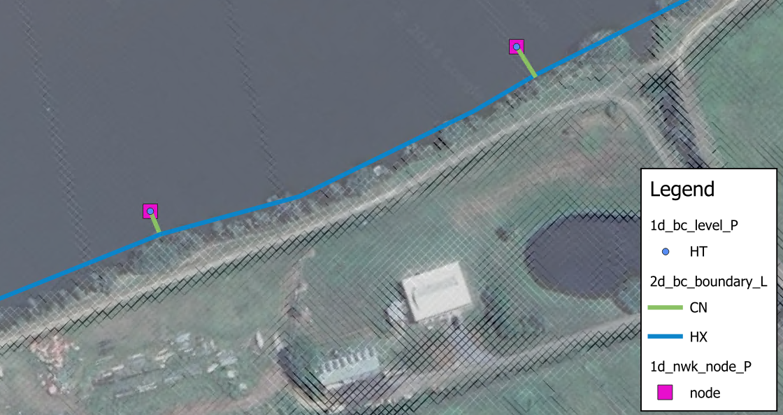
Figure 8.1: Sloping Water Level Boundaries

8.4.1.2 Groundwater Boundaries

At the edges of the active model area, three boundary conditions are currently supported for the groundwater layers:

1. Sealed boundary, no inflow or outflow (default in absence of defined boundary);
2. Groundwater level vs time (type “GT”) as detailed in Table 8.5; and
3. Source flow from a 1D model (type “SX”) as detailed in Table 8.6. See Section 10.2.2.2.

To specify a groundwater level vs time boundary, a “GT” type boundary line can be digitised in the 2d_bc file format. The same groundwater level boundary applies to all vertical layers. If the specified groundwater level is below the elevation at the bottom of the layer, it is dry. If the specified groundwater level is above the elevation at the top of the layer, the layer is fully saturated.

8.4.2 Source Area Boundaries

A 2d_sa layer is used to define a Source – Area boundary (flow or rainfall vs time), applying the flow directly onto the cells within the digitised polygon. Negative values remove water directly from the cell(s). There are multiple options regarding these boundaries:

• Source - Area boundary (2d_sa) - see Section 8.4.2.1 for options to spatially distribute applied flows.
• Source - Area Rainfall boundary (2d_sa_rf) - see Section 8.4.2.2 for specifying an input rainfall hyetograph instead of flow hydrographs.
• Source - Area Trigger option (2d_sa_tr) - see Section 8.4.2.3 for initiating inflow hydrographs based on a flow or water level trigger.
• Source - Area Flow option (2d_sa_po) - see Section 8.4.2.4 for modelling seepage or infiltration based on a varying water level or flow rate elsewhere in the model.

8.4.2.1 Source Area Options (2d_sa)

There are a number of options for distributing flows to cells within a SA region, these are:

• Distributed firstly to the lowest cell and then distributing between wet cells (Read GIS SA). This is the default option.
  
• Distributed to 2D cells connected to 1D pits (Read GIS SA PITS).
  
• Distributed to all cells equally (Read GIS SA ALL).
  
• Distributed to streamlines when used in conjunction with (Read GIS SA STREAM ONLY). The default option is to distribute SA inflows to all streamline cells and any non-streamline wet cells. This can be further controlled with Read GIS SA STREAM ONLY or Read GIS SA STREAM IGNORE.

The cells that the SA polygons are applying flow to can be checked using the _sac_check layer.

Any one of these options for spatially distributing flow can be used in combination with any one of the other special options (“RF” - Section 8.4.2.2, “TRIGGER” - Section 8.4.2.3 and “PO” - Section 8.4.2.4.

When distributing the water between the cells there are two options that can be specified in the .tcf. These are:

• SA Minimum Depth, this sets a minimum depth below which flow will not be distributed to the cell (apart from the lowest cell). The default minimum depth is -99999 (i.e. 0 depth, representing a dry cell).
  
• SA Proportion to Depth, this command proportions the SA inflows according to the depth of water. The default is ON, which proportions the flow according to the depth of water in the cells with deeper cells getting more flow.

The PITS option directs the inflow to 2D cells that are connected to a 1D pit or node connected to the 2D domain using “SX” for the Conn_1D_2D (previously Topo_ID) 1d_nwk attribute. The inflow is spread equally over the applicable 2D cells. An ERROR occurs if no 2D cells are found within the region.

The ALL option is available to apply the flow/rainfall to all active cells (either wet or dry cells) within the region. Not including any inactive or cells that have a water level boundary or HX 1D/2D linkage applied. If using the ALL option the double precision (see Section 13.3.2) version may be needed when using TUFLOW Classic as this is a similar approach to direct rainfall modelling.

The distribution of SA inflows to streamlines is activated when used in conjunction with Read GIS Streams command. This is discussed further in Section 8.4.2.1.1.

Table 8.7 lists the attributes for 2d_sa layers which are referenced in the .tbc file using the command Read GIS SA to read in flow hydrographs

Models using the Read GIS SA functionality are provided in the Inflows Example Model Dataset on the TUFLOW Wiki.

Table 8.7: 2D Source over Area (2d_sa) Attribute Descriptions

No.	Default GIS Attribute Name	Description	Type
1	Name	The name of the BC in the BC Database (see Section 8.5). The 2023-03 release changes the behaviour of HPC and Classic models that use multiple SA polygons with the same boundary name. In the 2023-03 release or newer, these boundaries are treated separately; as if they were different boundary names with the same hydrograph. Previously, these SA boundaries would be treated as a single boundary and the cells selected by each polygon would be grouped together. If duplicate SA boundary names are encountered, TUFLOW will issue CHECK 2492 in the 2023-03 Release.	Char(100)

8.4.2.1.1 Streamlines

Streamlines allow the user to apply SA inflows along the waterways rather than to the lowest cell (when all cells are dry within the SA region). This approach can be useful to apply baseflows to a river channel for instance. If streamlines have been specified using the .tbc Read GIS Streams command, SA inflows are distributed along the 2D cells selected by the stream lines within each SA region.

Read GIS Streams can be used one or more times in the .tbc file to define streamline cells. Streamlines are line objects, usually representing the path of the waterways. One attribute is required, which is the Stream Order as an integer type, as shown in Table 8.8. Only objects with a Stream Order greater than zero (0) are used by TUFLOW. Streams that are not to be used for applying SA inflows can be assigned a stream order of 0 (or deleted from the layer). The 2D cells along a streamline are selected as a series of continuous cells in the same manner as any other boundary line.

GIS and other software have the ability to generate streamlines from DEMs, and usually assign a stream order to each stream line. If needed, rearrange (or copy) the attributes so that the first attribute is the specified stream order. Alternatively, use the ‘Insert TUFLOW Attributes to existing GIS layer’ tool within the QGIS TUFLOW Plugin.

By default, any wet cells that are not streamline cells are also included in the distribution of the SA inflow. The commands Read GIS SA STREAM ONLY and Read GIS SA STREAM IGNORE provide options for controlling streamline inflows.

The _sac_check layer will show those cells selected as streamline cells.

Table 8.8: Streamlines (2d_strm) Attribute Descriptions

No.	Default GIS Attribute Name	Description	Type
1	Stream Order	The stream order. Objects with a stream order greater than 0 are used.	Integer

8.4.2.2 Rainfall Option (2d_sa_rf)

Read GIS SA RF (rainfall) option calculates flow from an input rainfall hyetograph based on catchment area, initial loss and continuing loss information specified in the 2d_sa_rf GIS file. Boundary condition inputs are specified as a rainfall hyetograph (mm versus hours) instead of flow hydrographs, which is required for the other Read GIS SA options.

Initial and continuing loss values applied through the Materials Definition file (.tmf or .csv format) are ignored when using the Read GIS SA RF (rainfall) option.

Models using the Read GIS SA RF functionality are provided in the Inflows Example Model Dataset on the TUFLOW Wiki.

Table 8.9: 2D Source over Area Rainfall (2d_sa_rf) Attribute Descriptions

No.	Default GIS Attribute Name	Description	Type
1	Name	The name of the BC in the BC Database (see Section 8.5). The 2023-03 release changes the behaviour of HPC and Classic models that use multiple SA polygons with the same boundary name. In the 2023-03 release or newer, these boundaries are treated separately; as if they were different boundary names with the same hydrograph. Previously, these SA boundaries would be treated as a single boundary and the cells selected by each polygon would be grouped together. If duplicate SA boundary names are encountered, TUFLOW will issue CHECK 2492 in the 2023-03 Release.	Char(100)
2	Catchment_Area	Additional attribute for the RF Option (Read GIS SA RF Command). The contributing catchment area in m2 (if using SI units) or miles2 (if using Units == US Customary). Note: This attribute is required as the polygon area is not used as the sub-catchment area because the rainfall area may be different to the polygon extent. A value of zero will trigger ERROR 2460.	Float
3	Rain_Gauge_Factor	A multiplier that allows for adjusting the rainfall due to spatial variations in the total rainfall. A value of zero will cause ERROR 2460 and the simulation will halt, see also Zero Rainfall Check command.	Float
4	IL	The Initial Loss amount in mm on inches (if using Units == US Customary).	Float
5	CL	The Continuing Loss rate in mm/hr or inches/hr (if using Units == US Customary).	Float

8.4.2.3 Trigger Option (2d_sa_tr)

Read GIS SA TRIGGER option allows the initiation of inflow hydrographs based on a flow or water level trigger. For example, reservoir failures can be initiated based on when the flood wave reaches the reservoir. An example of this option is:

Read GIS SA Trigger == gis\2d_sa_tr_dambreaks.shp

The 2d_sa_tr layer is a 2d_sa layer (with one attribute, Name), to which three additional attributes are added, as listed in Table 8.10. These are:

• Trigger_Type
  
• Trigger_Location
  
• Trigger_Value

Every timestep during the simulation, the flow (Q_) or water level (H_) of the 2d_po object referenced by Trigger_Location is monitored. When the 2d_po exceeds the Trigger_Value value the SA hydrograph commences.

If applying the hydrograph as a dam break, when digitising the SA trigger polygon, it should preferably be on the downstream side of the dam wall, extending the width of the dam wall and possibly be several cells thick (in the direction of flow). If there are stability issues, enlarging the SA polygon will help, however applications have indicated the feature typically performs well with the SA polygon a few cells thick.

The 2d_po line (flow) or point (water level) referred to by Trigger_Location can be located anywhere in the model. For cascade reservoir failure modelling it would usually be modelled using a 2d_po flow line, or for a 2d_po water level point just upstream of the dam.

Note: 2d_po flow lines MUST be digitised from LEFT to RIGHT looking downstream (if not, the flow across the 2d_po line will be negative and the trigger value will never be reached).

Table 8.10: 2D Source over Area Trigger (2d_sa_tr) Attribute Descriptions

No.	Default GIS Attribute Name	Description	Type
1	Name	The name of the BC in the BC Database (see Section 8.5). The 2023-03 release changes the behaviour of HPC and Classic models that use multiple SA polygons with the same boundary name. In the 2023-03 release or newer, these boundaries are treated separately; as if they were different boundary names with the same hydrograph. Previously, these SA boundaries would be treated as a single boundary and the cells selected by each polygon would be grouped together. If duplicate SA boundary names are encountered, TUFLOW will issue CHECK 2492 in the 2023-03 Release.	Char(100)
2	Trigger_Type	Trigger_Type must be set to “Q_” or “Flow” for a trigger based on a flow rate, or “H_” or “Level” for a trigger based on a water level.	Char(40)
3	Trigger_Location	Trigger_Location is the PO Label in a 2d_po layer (see Section 11.3.2.1). The 2d_po Type attribute must also be compatible with the Trigger_Type (i.e. it must include Q_ or H_ as appropriate).	Char(40)
4	Trigger_Value	Trigger_Value is the flow or water level value that triggers the start of the SA hydrograph.	Float

8.4.2.4 Flow Feature (2d_sa_po)

The Read GIS SA PO option models seepage or infiltration based on a varying water level or flow rate elsewhere in the model. This functionality is available when using TUFLOW Classic only. For example, modelling the seepage of groundwater into a coastal lagoon that is dependent on the water level in the lagoon.

The feature is set up as follows:

1. Create a 2d_po point object of Type “H_” at the water level location.
   
2. Add “Read GIS PO == …” to the .tcf file if not already there.
   
3. Create a new 2d_sa_po layer, as listed in Table 8.11. As of the 2023-03-AF release this layer is automatically created when using the Write Empty GIS Files command, previously this layer had to be created manually by adding the two following attributes to a 2d_sa layer:
   1. PO_Type: Char of length 16
      
   2. PO_Label: Char of max length 40
      
4. Digitise the SA polygon(s) covering the area of seepage or infiltration and for the attributes:
   1. Set the Name attribute to the name of the water level vs flow curve in the BC database.
      
   2. Set PO_Type to “H_”.
      
   3. Set PO_Label to the PO Label of the relevant 2d_po “H_” point to be used to determine the flow from the h vs Q curve.
      
5. Add “Read GIS SA PO == …” to the .tbc file.

Alternatively, to base the SA flow on the flow elsewhere in the model, use a 2d_po line object of Type “Q_”. To check the SA in/outflow:

1. View the _MB.csv files. The SA in/outflow from the seepage or infiltration will be part/all of the SS columns.
   
2. Add “SS” to the Map Output Data Types command. This outputs the net in/outflow from all source flows (ST, SA, SX and rainfalls) over time.

Table 8.11: 2D Source over Area Flow Feature (2d_sa_po) Attribute Descriptions

No.	Default GIS Attribute Name	Description	Type
1	Name	The name of the BC in the BC Database (see Section 8.5). The 2023-03 release changes the behaviour of HPC and Classic models that use multiple SA polygons with the same boundary name. In the 2023-03 release or newer, these boundaries are treated separately; as if they were different boundary names with the same hydrograph. Previously, these SA boundaries would be treated as a single boundary and the cells selected by each polygon would be grouped together. If duplicate SA boundary names are encountered, TUFLOW will issue CHECK 2492 in the 2023-03 Release.	Char(100)
2	PO_Type	PO_Type must be set to “Q_” to set the SA flow in/out of a model based on a flow rate, or “H_” to base it on a water level.	Char(16)
3	PO_Label	PO_Label is the Label attribute in a 2d_po layer (see Section 11.3.2.1). The 2d_po Type attribute must also be compatible with the PO_Type (i.e. it must include Q_ or H_ as appropriate).	Char(40)

8.4.2.5 Overlapping 2d_sa/2d_rf regions

2d_sa regions and 2d_rf regions introduced in the subsequent section (8.4.3.1.3) may overlap and their respective source terms apply cumulatively on a cell by cell basis. With the TUFLOW Classic solution scheme there is no limit to the number of regions that stack up (i.e. overlap) at a given location. However, for the TUFLOW HPC scheme (including Quadtree), the total number of 2d_sa and 2d_rf regions that apply at a given cell is limited to 4. The stack depth is checked at each cell and ERROR 2443 will result if the limit is exceeded.

8.4.3 Rainfall Boundaries

While the 2d_bc (Section 8.4.1) and 2d_sa (Section 8.4.2) approaches require users to predefine inflow hydrographs at model boundaries based on monitoring data or extracted from external hydrologic modelling tools, rainfall depth can be applied directly to 2D cells across the entire catchment to simulate catchment runoff. This direct rainfall approach enables the integration of catchment hydrology and hydraulic modelling within a single framework.

Four approaches are available for applying rainfall directly to the 2D cells. These are listed below and described in the following sections.

• Global Rainfall: the same rainfall is applied uniformly across the entire model domain.
• Rainfall Polygons (2d_rf): the model domain can be subdivided into a series of user-defined rainfall polygons, each assigned spatially uniform rainfall from a different gauge.
• Rainfall Control File (.trfc): rainfall gauges are defined as point locations, and a series of commands are applied to control the spatial interpolation of rainfall across the model domain. This approach generates a series of rainfall grids available to the user for display or checking.
• Gridded Rainfall: rainfall distribution over time applied as a temporally indexed series of grid files (.tif, .flt, .asc) or in a NetCDF file.

8.4.3.1 Rainfall Boundary Configuration

8.4.3.1.1 Rainfall Data

For all rainfall boundaries (except Gridded Rainfall), the input data must be prepared in a hyetograph format, and referenced in the BC Database (bc_dbase - Section 8.5). The rainfall data must be in simulation time (hours) versus depth (mm) (or time versus inches if using Units == US Customary). Time increments do not have to be a constant interval. The input data is converted to rainfall rate (mm/h or in/h) and, by default, is applied using a STEPPED approach, which holds the rainfall rate constant for the time interval.

The first and last rainfall entries should be set to zero, otherwise these rainfall values are applied as a constant rainfall if the simulation starts before or extends beyond the first and last time values in the rainfall time-series.

In Figure 8.2 below, the rainfall depth of 4.0mm is applied between the simulation times of 0hr and 0.25h, as a constant rainfall rate of 16.0mm/h, while the rainfall depth of 6.1mm is applied between the simulation times of 0.25h and 0.5h, as a constant rainfall rate of 24.4mm/h.

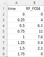
Figure 8.2: Example Rainfall Data Hyetograph

Note that SMOOTH approach can be applied to some rainfall BC (boundary condition) types. Please refer to the Rainfall Boundaries command in Appendix A.

8.4.3.1.2 Global Rainfall

The .tbc command Global Rainfall BC may be used to apply a spatially uniform rainfall depth to all active cells within the 2d_code layer based on the input hyetograph.

Global Rainfall BC == <rainfall_bc_name>

<rainfall_bc_name> is the name of the boundary condition (BC) in the BC Database (see Section 8.5).

Global Rainfall Initial Loss and/or Global Rainfall Continuing Loss can be used to quickly set up the rainfall losses for the Global Rainfall option. These commands must be set prior to the Global Rainfall BC command.

However, note that if losses are also specified in the Materials file (see Section 7.2.7.3 and Section 7.2.7.4), the material based losses are preferentially applied over the global loss options. See Section 8.4.3.1.6 for information on rainfall losses.

Global Rainfall Area Factor can be used to factor the global rainfall after the application of global losses, and otherwise before the application of materials file losses.

An example of global direct rainfall model is provided in TUFLOW Module 6 - Part 1.

8.4.3.1.3 Rainfall Polygons

The 2d_rf GIS layer applies a rainfall depth to every active cell within the digitised polygon using the Read GIS RF command, based on an input hyetograph.

Read GIS RF == <path_to_2d_rf>

Table 8.12 lists the attributes in 2d_rf layers.

The 2d_rf layer effectively utilises the digitised polygon extent as the “contributing catchment area”. This differs to 2d_sa_rf approach (Section 8.4.2.2) which requires a catchment area to be manually specified.

An example direct rainfall model using rainfall polygons is provided in TUFLOW Module 6 - Part 2.

Table 8.12: 2D Direct Rainfall over Area (2d_rf) Attribute Descriptions

No.	Default GIS Attribute Name	Description	Type
1	Name	The name of the rainfall BC in the BC Database (see Section 8.5). It is recommended that each polygon has a unique Name and that they do not overlap.	Char(100)
2	f1	A multiplier that allows for adjusting the rainfall due to spatial variations in the total rainfall. To vary the rainfall spatially, apply different f1 and/or f2 attribute values to each polygon. Values of f1 greater than 1 are permitted but, a value of zero will cause ERROR 2460 and the simulation will halt. See also Zero Rainfall Check command.	Float
3	f2	A second multiplier that allows for adjusting the rainfall spatially. Values of f2 greater than 1 are permitted but, a value of zero will cause ERROR 2460 and the simulation will halt. See also Zero Rainfall Check command.	Float

8.4.3.1.4 Rainfall Control File (.trfc)

Where the 2d_rf Rainfall Polygon applies spatially uniform rainfall inside the polygons, a Rainfall Control File (.trfc) contains a series of commands that can be used to both temporally and spatially interpolate the rainfall from rainfall gauges, generating pre-processed rainfall grids. Appendix F contains the full list of required and optional .trfc commands.

The .trfc file can be read in the .tcf file using the following command:

Rainfall Control File == <path_to_.trfc>

Note: Only one .trfc file can be specified in the .tcf file.

As with the Global Rainfall and the 2d_rf Rainfall Polygons, the rainfall distribution varies over time according to the input hyetographs at the gauges (Section 8.4.3.1.1).

Three methods are available to spatially interpolate rainfall depths from the gauges to the 2D domain. The following .trfc command is used to set the interpolation method. This command is compulsory as there is no default interpolation method.

RF Interpolation Method == IDW | POLYGON | TIN

• IDW (Inverse Distance Weighting)

  Rainfall depth is calculated based on the distance to the surrounding rainfall gauges, specified in 2d_rf format (see Table 8.12) by the following command:

  Read GIS RF Point == <path_to_2d_rf_point_file>

  The calculation is done via the inverse distance weighting approach:

  \[\begin{equation} z_{r} = \frac{\sum_{i = 1}^{n} (\frac{z_{i}}{d_{i}^{p}})}{\sum_{i = 1}^{n} (\frac{1}{d_{i}^{p}})} \tag{8.2} \end{equation}\]

  Where:

  • \(z_{r}\) = interpolated rainfall depth at a specific location
  • \(z_{i}\) = rainfall depth at rainfall gauge \(i\)
  • \(d_{i}\) = distance to rainfall gauge \(i\)
  • \(p\) = exponent used in IDW interpolation (default value is 2)
  • \(n\) = maximum number of rainfall gauges used in IDW interpolation

  The exponent (\(p\)) can be changed from its default value of 2 using IDW Exponent. The IDW Maximum Points and IDW Maximum Distance can be used to exclude points from the interpolation, this can reduce memory requirements when a large number of rainfall points are used. If using, it is strongly recommended to adjust IDW Maximum Distance and IDW Maximum Points based on the spatial density of the rainfall gauges in the model domain to ensure sensible rainfall distribution is generated from the IDW interpolation.

  If null value exists in the rainfall input data, the following .tcf command can be used to exclude the null data for the IDW rainfall interpolation:

  Rainfall Null Value == {-99} | <null_value>

• TIN (Triangulation Irregular Network)

  TIN interpolation is applied to calculate rainfall depth. The rainfall gauges are specified in 2d_rf format (see Table 8.12) by the following command:

  Read GIS RF Point == <path_to_2d_rf_point_file>

  While a TIN used for spatial interpolation is specified via the following command:

  Read GIS RF Triangles == <path_to_tin>

  The TIN polygons must connect the rainfall point (Read GIS RF Point) using triangles. No attribute is required for the TIN file, as TUFLOW only checks for the polygon shape to conduct TIN interpolation.

• POLYGON

  Similar to the 2d_rf Rainfall Polygons method, a series of polygons in 2d_rf format (see Table 8.12) can be specified to apply spatially uniform rainfall within each polygon:

  Read GIS RF Polygons == <path_to_2d_rf_polygon_file>

  This can be used to apply distributions such as Thiessen polygons generated from other software. The Rainfall Control File (.trfc) approach is more memory efficient compared to the 2d_rf Rainfall Polygons approach. See discussion below for more information.

  Read GIS RF Point can optionally be specified in combination with Read GIS RF Polygons for the POLYGON interpolation method. In such cases, the rainfall gauges are specified by the Read GIS RF Point command with 2d_rf format (see Table 8.12), while the Rainfall Polygons (which must have blank Name attributes) are only used to define the area that each point rainfall gauge is applied to. Although this approach requires two input files, this can be useful when using the same point rainfall gauge file to compare the 3 spatial interpolation approaches in one control file. Expand the dropdown below for an example of this.

Example .trfc - Compare interpolation approaches

Read GIS RF Point == <path_to_2d_rf_point_file>
If Scenario == IDW
  RF Interpolation Method == IDW
  IDW Exponent == 2
  IDW Maximum Distance == <distance>
  IDW Maximum Points == <number_of_points>
Else If Scenario == TIN
  RF Interpolation Method == TIN
  Read GIS RF Triangles == <path_to_tin>
Else If Scenario == POLY
  RF Interpolation Method == POLYGON
  Read GIS RF Polygons == <path_to_2d_rf_polygon_file>
End If

The rainfall control file is processed during model initialisation. A series of rainfall grids are output into a new “RFG” folder in the same location as the .trfc file. These are then used by the simulation to vary the rainfall over the 2D domain(s). This rainfall grid pre-processing approach reduces memory usage whilst TUFLOW is running. The generated rainfall grids can be interrogated prior to the end of the simulation for checking purposes and are also useful for displaying purposes. The rainfall grid format must be specified in the .trfc file using the following mandatory command:

RF Grid Format == ASC | FLT | NC | TIF

For more details on the different formats, please see the RF Grid Format command in Appendix F.

By default, the grid size of the generated rainfall grids is 10 times the 2D domain cell size. The RF Grid Cell Size command can be optionally specified to adjust the spatial resolution and/or to reduce the file size.

Note, the generated rainfall grids are inclusive of adjustments made in the BC Database (e.g. multiplication factors used for climate change) and of spatially-dependent adjustment factors in the input GIS layer’s attributes. They are not inclusive of the Rainfall Boundary Factor and any rainfall losses that may be specified in a materials file, which are applied during the simulation. The generated grids, either the NetCDF or the non-NetCDF formats with a csv file, can be utilised as Gridded Rainfall inputs for subsequent simulations to save the pre-processing time.

An example of a total rainfall depth grid, output when using the .trfc IDW interpolation approach and four rainfall gauges, is shown in Figure 8.3.

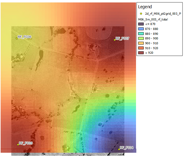
Figure 8.3: Example Depth Total Grid

Example .trfc files are available in the TUFLOW Wiki Rainfall Control File Examples and in TUFLOW Tutorial Module 6 - Part 3.

8.4.3.1.5 Gridded Rainfall

If the rainfall data is already prepared in grid format, it may be applied to the model using the .tcf command Read Grid RF. The command references a .csv index containing links to rainfall grids or a NetCDF file containing the time-varying data.

Read Grid RF == <path_to_rainfall_database_file>

or,

Read Grid RF == <path_to_rainfall_netcdf_file>

This allows the applied rainfall to vary spatially across the model without digitising multiple rainfall polygons within a 2d_rf GIS layer (Rainfall Polygons approach). If using the .csv file index, the rainfall grids may be in any TUFLOW supported grid format (.tif, .flt, .asc), noting that .tif and .flt are much faster for TUFLOW to process than .asc.

To use the NetCDF format, please refer to TUFLOW NetCDF Rainfall Format Wiki Page.

For the .csv index format, the rainfall database contains two columns, the first being time (in simulation hours) and the second being the rainfall grid (total rainfall depth for the time increment in mm). Time increments do not have to be a constant interval. The indexed grids are converted to rainfall rate (mm/h or in/h), and applied using a STEPPED approach, which holds the rainfall rate constant for the time interval.

An example of a rainfall database is shown in Figure 8.4. In this example, the values in the 2^nd rainfall grid are the total rainfall depth from time 0 to time 0.17 hours (i.e. not the rainfall intensity in mm/h or inch/h). In the first and last rainfall grid, the rainfall depth is recommended to be set to zero. Otherwise, the rainfall rates calculated based on the first/last rainfall grids are extended before and after the first/last rainfall grid times in the .csv file, if the simulation starts before or extends beyond the first and last time grid time.

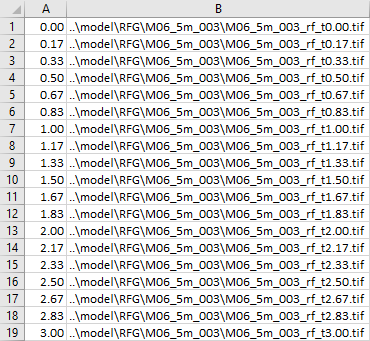
Figure 8.4: Example Rainfall Database

An example direct rainfall model using rainfall grids is provided in TUFLOW Tutorial Module 6 - Optional.

8.4.3.1.6 Rainfall Losses and Infiltration

TUFLOW supports a range of rainfall loss and soil infiltration options. The following loss and infiltration methods are listed in order of processing application:

• The rainfall loss approach is a simplistic calculation method comparable to the rainfall excess loss methods included in traditional hydrology models, typically representing evapotranspiration or interception losses. In TUFLOW, rainfall losses remove the loss depth from the rainfall depth, before it is applied as a boundary to the 2D cells. Rainfall losses can be defined via:
  • Global losses: Global Rainfall Initial Loss and Global Rainfall Continuing Loss (Section 8.4.3.1.2) can be applied for Global Rainfall only, in the absence of materials-based losses below.
  • Materials-based losses: Initial and continuing losses can be defined in the materials file and applied spatially based on the material types (see Section 7.2.7.3).
  • SCS Curve Number loss approach (USDA, 1986): Estimates rainfall excess losses as a function of cumulative precipitation, soil cover, land use, etc. In TUFLOW, the SCS infiltration parameters are set based on soil type (see Section 7.3.5.1.1).
• Soil Infiltration:
  • Various soil infiltration approaches (e.g. Green-Ampt, Horton and ILCL, see Section 7.2.8) infiltrate ponded water into the soil after rainfall is applied to the 2D cells. This is considered a more realistic representation of the actual physics and is recommended when using direct rainfall modelling.

Note: rainfall losses are not applied to negative rainfall values (e.g. to model evaporation), see Section 8.4.3.8.

8.4.3.1.7 Rainfall Adjustments

During sensitivity testing or for factoring rainfall intensity for scenarios such as climate change, rainfall can be easily adjusted via a number of different methods, instead of rewriting the input hyetograph:

• bc_dbase adjustments can be made for the Global Rainfall, 2d_rf Rainfall Polygons and Rainfall Control File (.trfc) approaches (see Table 8.13).
• Rainfall Boundary Factor can be used to apply a global multiplication factor for all rainfall boundary types. This factor compounds with any initial bc_dbase adjustments.
• 2d_rf layer adjustments can be made with the F1 and F2 attributes for 2d_rf Rainfall Polygons and Rainfall Control File (.trfc) boundaries (see Table 8.12).

Note: These rainfall adjustments are applied before rainfall losses (Section 8.4.3.1.6).

• Global Rainfall Area Factor can be set for Global Rainfall boundaries only, factoring rainfall after the subtraction of any Global Rainfall Initial Loss or Global Rainfall Continuing Loss.

8.4.3.2 Checks and Results

8.4.3.2.1 Check Files

The 2d_bc_tables check file provides rainfall data inclusive of any bc_dbase adjustments only for Global Rainfall and 2d_rf Rainfall Polygon boundaries (Section 8.4.3.1.3).

The TUFLOW Log File (.tlf, see Section 14.4.1) provides the following processed rainfall data. Key phrases to search in the .tlf to locate the data are provided in italics.

• For Global Rainfall, processed rainfall data, inclusive of:
  • any bc_dbase adjustments and Rainfall Boundary Factor (search .tlf: Rainfall histogram after rain gauge factor adjustment);
  • then global losses (search .tlf: Rainfall histogram conversion after IL and CL);
  • then Global Rainfall Area Factor, and converted to mm/h (or in/h) (search .tlf: Global Rainfall histogram).
• For 2d_rf Rainfall Polygons boundaries, processed rainfall data, inclusive of:
  • any bc_dbase adjustments and Rainfall Boundary Factor (search .tlf: Rainfall histogram after Rainfall Boundary Factor adjustment);
  • then converted to mm/h (or in/h) (search .tlf: RF Rainfall histogram conversion).
• For Rainfall Control Files (.trfc), the processed rainfall data are reported in the .tlf inclusive of bc_dbase adjustments and spatially-dependent adjustment factors in the input GIS layer’s attributes (search .tlf: Rainfall histogram after rain gauge factor adjustment).

For Rainfall Control Files (.trfc), rainfall depth grids are also generated during preprocessing. These grids are inclusive of bc_dbase adjustments (e.g. multiplication factors used for climate change) and of spatially-dependent adjustment factors in the input GIS layer’s attributes, but exclusive of Rainfall Boundary Factor and any materials file rainfall losses. These can be interrogated prior to the end of simulation.

Note, to use US customary units, the .tcf command Units == US Customary must be specified.

8.4.3.2.2 Map Outputs

It is recommended to activate several Map Output Data Types specific to direct rainfall modelling (See Table 11.4) for model diagnostic and display purpose, including:

• RFR and RFC: view the rainfall rate (mm/h or in/h) and cumulative rainfall (mm or in) over time respectively. These are inclusive of rainfall adjustments and losses and can be used as additional checks.
• RFML: spatially view the cumulative materials file based rainfall losses (mm or in).
• CI and IR: Cumulative Infiltration (mm or in) and infiltration rate (mm/h or in/h) applied based on the soil infiltration calculation.

As a direct rainfall model applies water to all 2D cells, it is also recommended to apply Map Cutoff Depth and Map Cutoff Vector to facilitate fit-for-purpose mapping that limits the display of user defined shallow depths.

Note, to use US customary units, the .tcf command Units == US Customary must be specified.

8.4.3.3 Wetting and Drying

As direct rainfall model applies rainfall across all the 2D cells within the whole catchment, a substantial number of cells could experience shallow sheet flow. It is recommended to consider reducing Cell Wet/Dry Depth from the default 0.002m (or 0.007ft) to less than a mm (e.g. 0.0002m or 0.0007ft) to invoke momentum calculation at the cell side at shallow depth.

Cell Wet/Dry Depth == 0.0002

This is recommended for both Classic and HPC solution schemes, unless using SGS. For HPC models with SGS enabled, lowering the Cell Wet/Dry Depth is not necessary, as the wetting/drying occurs in the SGS storage curve (Section 8.4.3.6).

Since the 2026.0.0 TUFLOW release, HPC Infiltration Drying Approach == Method C is the default infiltration approach in the HPC solver to improve the model stability. TUFLOW dries cells (switches off momentum calculation) once the cell water depth falls below the cell wet/dry depth. However, Method C allows soil infiltration to occur in dry cells with positive rainfall rate, until the depth reaches a smaller depth. The first threshold to switch off momentum calculation (or the ‘wetting depth’ in the image below) is still set by the Cell Wet/Dry Depth command. The second threshold to switch off infiltration (or the ‘drying depth’) is set by the HPC Infiltration Drying Depth command.

This command is optional. If omitted, the default drying depth is Cell Wet/Dry Depth - 0.0001m (or 0.0001ft if using Units == US Customary).

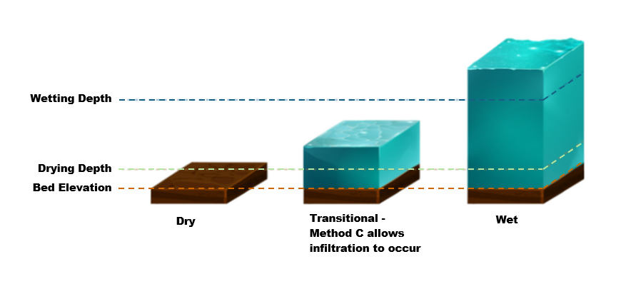
Figure 8.5: Default HPC Infiltration Approach (Method C)

8.4.3.4 Bed Roughness for Direct Rainfall Model

In a direct rainfall model, sheet flow occurring over steep terrain can lead to a break down of key assumptions applied in the conventional shallow water equation (SWE):

• Conventional SWE solvers assume a small bed slope and does not account for slope angle in the pressure term for steeper terrain.
• The Manning’s coefficient is usually derived for deep flow in channels where the roughness elements are very small compared to the flow depth. Manning’s n value and/or equation may not be a reliable estimate of bed resistance at the shallow sheet flow depths typical to direct rainfall modelling, where higher roughness values relative to the shallow depth are expected.

It is highly recommended to adjust the Manning’s n values to calibrate the hydraulic response of catchments. Application of depth varying roughness (see Section 7.2.7.3) or “Law of the Wall” approach (Section 7.2.7.2) can be also considered to take into account of the high roughness at shallow depth and/or to counter the overestimation of the pressure gradient in a direct rainfall model.

8.4.3.5 Model Precision and Memory Requirements

TUFLOW Classic uses an implicit finite difference solver for which the primary state variable is the water elevation. The use of water elevation as the primary variable can have limitations when run in single precision. When computing differences in water elevations between adjoining cells, numerical precision errors arise when the model has high altitude DEM data, or very thin sheet flow (i.e. rainfall models). When using TUFLOW Classic for models with high altitude and/or rainfall, it is advisable to run the model with the double precision executable, see Section 13.3.2. The .tcf command Model Precision == Double can be used to ensure that only a double precision version of TUFLOW is used.

TUFLOW HPC (including Quadtree) uses an explicit finite volume scheme based on water depth, and the single precision executable generally works well for models with high altitude and/or rainfall. If in doubt, or even just curious, it is recommended to re-run the same model in double precision and compare the results.

Note that switching to double precision also increases the memory footprint. This is usually not a constraint for direct rainfall models running on CPU. However, for HPC models running on GPU hardware, the increased memory footprint may become a constraint due to the limited onboard memory typically available on GPUs. For this reason, the ‘POLYGON’ interpolation approach (Section 8.4.3.1.4) defined using a Rainfall Control File (.trfc) is preferred over the direct rainfall boundary condition inputs defined using the 2d_rf Rainfall Polygon approach with the Read GIS RF command, as the former requires a far smaller amount of memory.

Also note that for non-high-performance GPU models (such as the GeForce series), simulation speed may reduce considerably when using double precision.

8.4.3.6 Sub-Grid Sampling (SGS) with Direct Rainfall

It is highly recommended to use HPC and sub-grid sampling (SGS), when modelling using direct rainfall. SGS represents cell storage and faces with a curve rather than flat elevations (see Section 7.3.3) and cells can be partially wet. SGS has been found to significantly improve direct rainfall modelling by low flow transmission of water with minimal retention or blocking of flows (Ryan et al., 2022) plus significantly reduced sensitivity to cell size (Kitts et al., 2020). See Section 3.2.3.1.

There are a number of associated SGS hydraulic calculation and output settings that should be reviewed for direct rainfall modelling given the differences in SGS vs standard flat cell schematisation and their interaction, particularly with shallow sheet flow. Please refer to the commands SGS Sheet Flow Approach, SGS Infiltration Approach and SGS Negative Rainfall Approach in Section 7.3.3.1.3 for more information.

8.4.3.7 Groundwater

Flood modelling of single rainfall event often requires considering soil infiltration and soil capacity. However, for long term continuous simulations with multiple rainfall events, it is recommended to enable the advection of groundwater flow to take into account the change in groundwater storage during dry periods. For more details please refer to the Section 7.3.5.2.

Also relevant to direct rainfall modelling with groundwater flow:

• Section 8.4.3.1.6 for information on soil based losses and infiltration, and
• Section 8.4.3.3 for information on the HPC infiltration drying approach.

8.4.3.8 Negative Rainfall

Negative rainfall values can be applied in TUFLOW to model evaporation/evapotranspiration. It is typically implemented as a negative Global Rainfall boundary overlapped with another type of inflow rainfall boundary (e.g. Global Rainfall + .trfc Rainfall Control File). Initial and continuing losses (Section 8.4.3.1.6) are not applied to negative rainfall values.

For groundwater enabled models, negative rainfall is allowed to be drawn from the topmost groundwater layer under surface layer cells that are dry, thus mimicking evapotranspiration (see Section 7.3.5.2.7). Prior to the 2023-03 release, this would only decrement the water in wet cells until they dry and would not draw from the cumulative infiltration layer.