Section 2 2D Domain Construction

2.1 Quadtree Updates (HPC Only)

The Quadtree mesh refinement functionality, added in the 2020-01 Release, allows the user to vary the resolution of a model using the HPC 2D Solver. The following enhancements have been included in the 2023-03 Release.

2.1.1 Support for Multiple GPU

Multiple GPUs are supported for the 2023-03 Release when using a quadtree mesh. For the 2020 Releases, only a single GPU per simulation could be utilised when using quadtree refinement. The functionality for multiple GPUs with Quadtree is the same as for a standard (single resolution) HPC model.

Device IDs can be specified in either the .tcf using the “GPU Device ID ==” command, or via the command line with -pu arguments. Device weightings can be specified with the “HPC Device Split ==” .tcf command (refer to Section 8.4 in the 2020 Release Notes).

As per standard HPC (without Quadtree) if peer-to-peer GPU access is available between GPU cards, via either an NVLink or via a compatible PCIe configuration, then this is utilised by default. This can be disabled with the command:

GPU Peer to Peer Access == DISABLED | {ENABLED IF AVAILABLE}

Note: With newer generations of GPUs increasing the CUDA cores and memory, multiple GPUs simulations will realistically be only confined to very large models.

2.1.2 Support for Multiple Nesting GIS Layers

The 2023-03 Release supports multiple 2d_qnl (nesting polygon) layers (i.e. multiple “Read GIS Nesting ==” commands in a single .qcf). Previously, TUFLOW would produce ERROR 2846 if more than one GIS nesting command was specified.

The order that the GIS layers are specified does not matter; TUFLOW will read in all GIS layers before processing the mesh. The exception to this is for level one nesting polygons where TUFLOW will adopt the last level one polygon that is found. Previously if more than one level one nesting polygon was found, ERROR 2825 was produced. This has been changed to WARNING 2825 and TUFLOW will override the previous level one polygon.

2.1.3 Support “Trigger 1D” for Variable Z Shape

The 2023-03 Release supports a “Trigger 1D” option for 2d_vzsh (variable Z shapes) to commence elevation updates based on the water level at a 1D node. The “Trigger 1D PF” can be used to trigger the elevation updates based on the progress of a 1D PF (Pipe Failure) channel.

2.2 Sub-Grid Sampling (SGS) Changes

Sub-Grid Sampling (SGS) stores and uses curves representing the sub 2D cell terrain data of the DEMs, TINs and Z shapes used to construct the model instead of each 2D cell and each 2D face having one elevation. This functionality was first introduced in the 2020-01 Release, the following changes to SGS functionality have been included in the 2023-03 Release.

2.2.1 SGS Default Changes

There have been several changes to the SGS defaults (if SGS is enabled with the .tcf command “SGS == On”) since the 2020-10 Release. These changes are listed in Table 2.1 and Table 2.2, discussed in the referenced sections.

Table 2.1: Changes in SGS Defaults

Command	2020 Default	2023 Default	Section
SGS Approach ==	Method B	Method C	Section 2.2.2
SGS Depth Output ==	Exact	Cell Average	Section 7.5.3 of the 2020 Release Notes
SGS Map Extent \(\langle\)Full or Trim\(\rangle\) ==	SGS Map Extent Full == h	SGS Map Extent Trim == ALL	Section 7.5.4 of the 2020 Release Notes
SGS Material ==	ON	OFF	Section 2.2.4

Table 2.2: Changes in HR Output Defaults

Command	2020 Default	2023 Default	Section
HR Interpolation Approach ==	Method A	Method C	Section 2.2.5
HR Thin Z Line Output Adjustment ==	OFF	ON CELL SIDES	Section 2.2.6

2.2.2 SGS Approach

For the 2023-03 Release “SGS Approach == Method C” is the default setting if SGS is enabled (SGS == ON). Method C was introduced as beta functionality in the 2020-10-AB Build. The previous default “SGS Approach == Method B” processed elevations into elevation-volume curves (for cells) and elevation-flow area/width curves (cell faces) after reading each elevation dataset. The sampled SGS elevations were discarded after processing the dataset for memory efficiency. Method C retains the SGS elevations in memory throughout the pre-processing stage and performs the generation of the curves only at the end of the pre-processing of all elevation data.

Whilst this can potentially use more memory (CPU RAM) the approach has considerable benefits in terms of preserving sub-grid elevation data at cells/faces partially affected by terrain data layers and allows TUFLOW to produce high-resolution mapping at the SGS sampling resolution.

See Section 3.7.2 in the 2020 Release Notes for details on the SGS Approach Method C.

2.2.3 Setting SGS Sampling Frequency

For the 2023-03 Release, when using the SGS Approach Method C (which is the default for Release 2023-03 – refer Section 2.2.1), there are now several ways of setting the SGS sampling frequency. For the 2020-10 Release when using SGS Method C, the SGS Sample Frequency had to be set using the .tcf command “SGS Sample Frequency == \(\langle\)number of sample locations per face\(\rangle\)”. For the 2023-03 Release, in addition to this command, it is also possible to alternatively set a sampling target distance using the new .tcf command:

SGS Sample Target Distance == \(\langle\)distance in metres or feet\(\rangle\)

TUFLOW requires an odd number of sample locations across a cell face to ensure the mid-point is a sample point. The sampling frequency is calculated as the TUFLOW cell size divided by the target distance then rounded as per Equation (2.1).

\[\begin{equation} \text{Sample Frequency} = \frac{\text{TUFLOW Cell Size}}{\text{Target Distance}} + 1 \tag{2.1} \end{equation}\]

For example, for a 10m TUFLOW model with a target distance of 1m, the sampling frequency is 11. Even numbers are rounded up to the next highest odd number. The sampling frequency adopted is reported in the .tlf.

If neither “SGS Sample Frequency ==” or “SGS Sample Target Distance ==” is set, a scan of the Geometry Control File (.tgc) is performed to find the minimum raster grid resolution used in “Read Grid Zpt ==” commands, and this is used as the sampling target distance to compute the sampling frequency. If there are no gridded elevation datasets, a default sampling frequency of 11 is used. In summary, there are four ways for the SGS Sample Frequency to be defined; in decreasing order of priority they are:

1. “SGS Sample Frequency ==” command.
2. “SGS Sample Target Distance ==” command.
3. Target distance automatically based on the minimum grid elevation resolution in the .tgc.
4. Default Sampling Frequency of 11 per face / 121 per cell.

Note: the sampling frequency is capped at 31 by default to avoid long pre-processing times and high memory usage. In general, a sampling frequency smaller than 31 is sufficient for most natural water ways or artificial structures, and users may not benefit from applying a super fine sample distance against the model cell size. However, if required, this upper limit can be increased by using the following tcf command:

SGS Max Sample Frequency == \(\langle\)maximum frequency\(\rangle\)

Note, a hard limit of 127 per face (16,129 samples per cell) still applies.

2.2.4 SGS Materials

For the 2023-03 Release the sub-grid sampling of materials (land-use) has been disabled. This functionality was included in the 2020-10 Release as beta functionality, see Section 3.7.3 of the 2020 Release Notes. Feedback and further testing indicates that additional development is required. Some significant issues have been identified including the large dynamic range in face depths over which the look-up table must be computed, the transition between sheet flow and channel flow, and the inclusion of the effects of eddy viscosity or sub-grid turbulence on the parallel flow analysis. The latter issue in particular needs further research to provide consistency between different cell sizes.

This feature is planned to be reinstated for an update to the 2023-03 Release once further research and benchmarking is completed.

2.2.5 High Resolution Interpolation Approach

For SGS Method C, the high resolution (HR) raster map output can be output at finer resolution than the 2D model size. It is important to note that this is interpolating cell centre / corners data across the cell. For the 2023-03 Release enhancements have been made to the interpolation approach.

Note: High resolution raster outputs are only available for depth (d) and water level (h) output data types.

For the 2020-10 Release this was beta functionality, see Section 3.7.4 of the 2020 Release Notes, and the only approach available is described below as “Method A”.

For models with traditional hydrology inflows, “Method A” generally produced effective HR maps. However, for models with very shallow flows (such as direct rainfall models), this could produce HR outputs with interpolation artefacts, as illustrated in Figure 2.1.

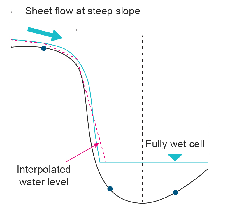
Figure 2.1: Linear Corner Interpolation for High Resolution Water Level at Steep Slope

“HR Interpolation Approach== Method B” improves this by introducing sheet flow checks when interpolating. “HR Interpolation Approach == Method C” uses the sheet flow checks and applies a weighting based on the number of wet SGS sampled locations in the cell.

Some example HR outputs for a model with direct rainfall and a very coarse 2D cell size are presented in Figure 2.2 to Figure 2.4.

“HR Interpolation Approach == Method C” is the default for the 2023-03 Release.

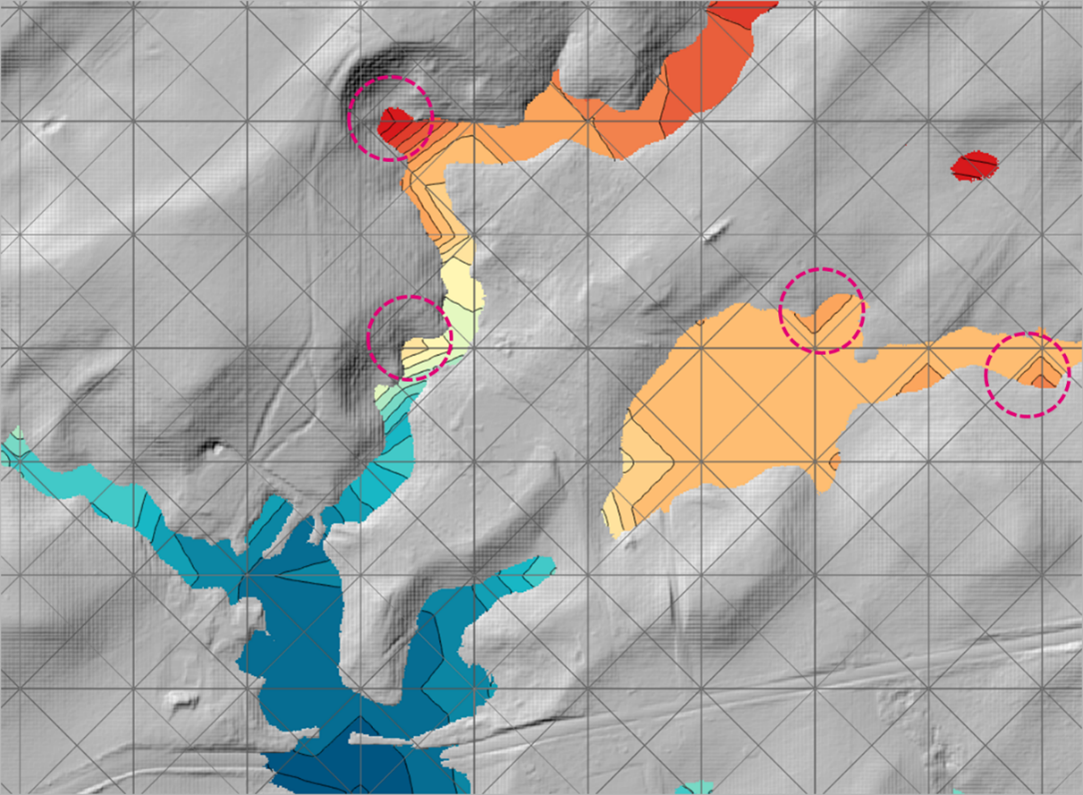
Figure 2.2: HR Interpolation Approach == Method A

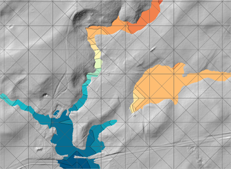
Figure 2.3: HR Interpolation Approach == Method B

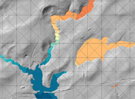
Figure 2.4: HR Interpolation Approach == Method C (new default)

2.2.6 High Resolution Thin Breaklines

When applying thin breaklines only the cell side and cell corner elevations are modified. For models with thin breaklines and HR outputs, the presence of breaklines can be used to affect the HR interpolation. A new .tcf command has been introduced to control this:

HR Thin Z Line Output Adjustment == OFF | {ON CELL SIDES} | ON ALIGNMENT

The three options provided are:

• OFF – Thin breaklines do not affect the HR raster interpolation
• ON CELL SIDES – This prevents interpolation across cell sides that have thin breaklines.
• ON ALIGNMENT – The location of the breakline within the TUFLOW cell resolution is stored and stops interpolation occurring over this topographic barrier.

“HR Thin Z Line Output Adjustment == ON CELL SIDES” is the default for the 2023-03 Release as this is consistent with the computational location which the topographic barrier is applied. Example outputs from a model with a thin breakline are shown in Figure 2.5 to Figure 2.7 for all three options.

Figure 2.5: HR Thin Z Line Output Adjustment == OFF

Figure 2.6: HR Thin Z Line Output Adjustment == ON CELL SIDES (new default)

Figure 2.7: HR Thin Z Line Output Adjustment == ON ALIGNMENT

2.2.7 Parallel Processing for SGS initialisation

As noted in Section 2.2.2, SGS Method C (the default if “SGS == On”) retains the SGS elevations in memory throughout the pre-processing stage and performs the generation of the curves only once at the end of the pre-processing. This is a computationally intense exercise, particularly for large models with small SGS sample distances. To speed up model initialisation, this has been configured to utilise multiple CPU cores.

By default, all CPU threads will be used for final SGS elevation pre-processing unless the number of threads (-nt[thread count]) command line argument has been specified. For example, to run on 8 threads the command line argument “-nt8” would be used. There is no check for thread licensing used for pre-processing. If the number of threads specified in the command line argument exceeds the number of threads available all threads are used.

See also computational and clock time updates in Section 8.8.

2.2.8 XF Files for SGS Method C

In addition to the parallelisation of the final SGS elevation pre-processing (described in Section 2.2.7), XF files are now supported for SGS Method C. At the end of the .tgc reading, after all elevation datasets have been processed, an XF file is written if the “XF Files ==” command is set to on (default).

The XF file is written to an “xf” folder which sits in the same location as the .tgc. To avoid re-processing when changes are made to .tgc data other than elevation (e.g. active cells, materials, soils, etc.), the XF file is not written with the same filename as the .tgc. Instead, the .xf will be prefixed by “hpc” or “qdt” for HPC and Quadtree simulations respectively and includes the nesting level, cell size. Any text set with the .tcf command “XF Files Include in Filename ==” is included.

When reading the pre-processed SGS XF file, a check is done on the final SGS elevations, if these are consistent then the XF file is used.

A fix was made to the XF file access check in the 2023-03-AD Build, see Section 8.4.1.

2.2.9 Enhancement for SGS Parameterisation

The 2023-03-AD build implements some enhancements for the SGS Parameterisation. Most of the changes are targeted at models that use the hydraulic radius to calculate the bed friction (“SGS Radius Approach == Hydraulic”). Note, this is not the default setting.

Some of the changes can cause minor differences in simulation results for SGS models regardless of SGS Radius Approach.

2.2.9.1 Enhancement in SGS Parameter Fitting

The 2023-03-AD release improves the SGS parameter fitting process at the cell faces. The improvements include:

• Better initialisation for the SGS parameters used to calculate the wetted perimeter vs height relationship.
  
• Improvements to the iteration process to minimise the fitting error.

Models using the default hydraulic resistant approach (“SGS Radius Approach == Resistance”) are not affected by the first change related to the parameter initialisation. However, the second change in fitting iteration can cause minor changes in the SGS parameters for a very limited number of cells, and thus result in marginal difference in modelling results for SGS models. These changes are considered to be bug fixes, and therefore no backward compatibility is provided.

Also due to the changes above, the SGS XF file version has been increased, and a new SGS XF file will be automatically generated when running models with Build 2023-03-AD.

2.2.9.2 Enhancement of Hydraulic Radius Implementation

The 2023-03-AD build improves the implementation of hydraulic radius for SGS models. When “SGS Radius Approach == Hydraulic” was used to calculate the bed friction prior to the 2023-03-AD build, TUFLOW could underestimate the flow resistance for steep-sided narrow channels. The new approach improves the hydraulic radius implementation to address this issue, and can be activated by using the following command:

“SGS Hydraulic Radius == Method B”

Note the default approach is “Method A” for backward compatibility. The models using the default hydraulic resistant approach are not affected by this change

2.2.10 Enhancement of Water Level Interpolation at BC Cells with Steep Bed Slope

Prior to the 2023-03-AD build, SGS models could generate a slight error in water level at boundary cells with steep bed slopes. This was caused by the HPC solver inadvertently using 1st order spatial interpolation at the boundary cell, while applying 2nd order spatial interpolation everywhere else. This issue can be addressed in the 2023-03-AD build by applying the following command:

SGS 2nd Order BC Slope == Method B

Note that this issue only occurs at BC cells with steep bed slopes (e.g. > 0.01), and doesn’t affect most real-world model boundaries. Therefore, ‘Method A’ (the original method) remains the default approach for backward compatibility.

2.3 Infiltration and Sub-Surface Flows

2.3.1 Overview

The 2023-03 Release permits horizontal flow of the water within the cumulative infiltration layer. Up to 10 vertical layers are supported, each with horizontal advection and vertical filtration from above. Movement of water within the ground in the real world is complex. The functionality introduced in the 2023-03 Release is not intended to replace detailed groundwater modelling, but provides a functional mechanism by which:

• Catchment response for 2D direct rainfall (“rain on grid”) models can be better calibrated to available river flow data.
• Long-term catchment models can be constructed that offer some prediction of stream flows long after rainfall events.
• The accuracy of real-time flood forecasts can be improved by taking into account the drying and draining of catchments that has occurred since the last rainfall event.
• Sub-surface seepage can cause inundation, such as seepage under a levee bank through a porous layer (e.g., old gravel river course), resulting in flooding on the protected side of the levee.

The basic concept is that of dividing the ground into vertical layers, each with a defined thickness (alternatively a z elevation for the bottom of the layer), soil type, and cumulative infiltration. The cumulative infiltration, combined with the porosity defined by the soil type, allows a theoretical “ground water elevation” (also known as a “water table”) to be computed within the layer as shown in Figure 2.8.

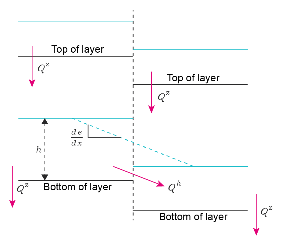
Figure 2.8: Interflow Concept

The vertical (or “convective”) flow of water from the surface water layer into the first (or top) ground water layer (also referred to as the interflow layer) is governed by the soil type infiltration model. The soil types in the top most layer must be one of those defined in Section 6.10 of the 2018 TUFLOW Manual. For layers below the first layer the vertical flow of water, \(Q^{z}\), is computed using a “convective” hydraulic conductivity (effectively the same concept as continuing loss):

\[\begin{equation} Q^{z} = - kdxdy \tag{2.2} \end{equation}\]

Where:

• \(k\) is the convective hydraulic conductivity
• \(dxdy\) is the cell area

This has required the addition of a new soil type “CO” for layers below the interflow layer.

The horizontal advection of water from one cell to the next, \(Q^{h}\), is computed using the horizontal hydraulic conductivity of the soil and the horizontal gradient of a variable called the “ground water pressure level”:

\[\begin{equation} Q^{h} = - k_{h}hp\frac{de}{dx}dy \tag{2.3} \end{equation}\]

Where:

• \(k_{h}\) is the horizontal hydraulic conductivity of the soil (average of the left and right cells used)
• \(h\) is the physical depth of water in the upstream cell (i.e. the ground water elevation less the layer bottom elevation)
• \(p\) is the soil porosity
• \(\frac{de}{dx}\) is the gradient of the “ground water pressure level”
• \(dy\) the width of the face.

For cells that are “unsaturated” the “ground water pressure level” is exactly the ground water elevation within that layer. For cells that are fully saturated, the ground water pressure level is that of the cell in the next layer above (or the water surface elevation if the next layer above is the surface layer). For cells that are “nearly saturated” the ground water pressure level is transitioned between these two options. The threshold at which the transition begins is called the “ground water blending threshold” (refer Section 2.3.8), \(\phi\).

\[\begin{equation} \xi = \frac{\frac{h}{dz} - \phi}{(1 - \phi)} \tag{2.4} \end{equation}\]

\[\begin{equation} e_{i} = (1 - \xi)\left( z_{i} + h_{i} \right) + \xi e_{i - 1} \tag{2.5} \end{equation}\]

\[\begin{equation} e_{0} = {WSE}_{surface} \tag{2.6} \end{equation}\]

Where:

• \(h\) is the depth of ground water in the cell
• \(dz\) the vertical thickness of the layer
• \(z_{i}\) the layer bottom elevation
• \(e_{i}\) the resulting ground water pressure level for the layer

The layer ordering is such that the surface water layer is “0”, the interflow layer is “1”, and any additional ground water layers range from 2 to N, from top to bottom.

If the sum of flows into a layer cell causes it to exceed its soil capacity, the excess is push upwards to the next layer. If this happens for the top-most interflow layer, the excess is pushed into the surface water layer as a “return flow”. This is to be expected in the creek beds but may also happen at the bottom of steep hills where the slope transitions from steep to shallow.

Although the above theory appears complex, the implementation within a TUFLOW model is straight forward. The essential steps are:

1. Read a soils (.tsoilf) data file from within the .tcf
2. Define layer thicknesses and soil types in the .tgc
3. Specify locations of groundwater boundaries
4. Add any additional output data types int the .tcf

These steps are explained in more detail in the following sections.

2.3.2 Soils File

The soils file (.tsoilf) may now include a new column of data for the horizontal hydraulic conductivity of the soils. If omitted, or if all soils used in the model have zero horizontal hydraulic conductivity, then horizontal advection of water will not be considered in the model. Additionally, a new soil type “CO” is required for any layers below the first (i.e. top or interflow) layer. The data columns for CO soils are detailed in Table 2.3.

Reading the .tsoilf file is the same as in previous Releases with the .tcf command “Read Soils File ==”.

Table 2.3: .tsoilf Parameters

Column No	No Infiltration	Green-Ampt	Green-Ampt	Horton	Initial / Continuing Loss	Convective
1	Soil ID	Soil ID	Soil ID	Soil ID	Soil ID	Soil ID
2	NONE	GA	GA	HO	ILCL	CO
3		USDA Soil Type (see Table 6-14)	Suction (mm or inches)	Initial Loss (mm or inches)	Initial Loss (mm or inches)	Hydraulic Conductivity (mm/h or in/h)
4		Initial Moisture (Fraction)	Hydraulic Conductivity (mm/h or in/h)	Initial Loss Rate (f0) (mm/h or in/h)	Continuing Loss (mm/h or in/h)	Porosity (Fraction)
5		Max Ponding Depth (m or ft)	Porosity (Fraction)	Final Loss Rate (fc) (mm/h or in/h)	Porosity (Fraction)	Initial Moisture (Fraction)
6		Horizontal Hydraulic Conductivity (mm/h or in/h)	Initial Moisture (Fraction)	Exponential Decay Rate (k) (h-1 )	Initial Moisture (Fraction)	Horizontal Hydraulic Conductivity (mm/h or in/h)
7			Max Ponding Depth (m or ft)	Porosity (Fraction)	Horizontal Hydraulic Conductivity (mm/h or in/h)
8			Horizontal Hydraulic Conductivity (mm/h or in/h)	Initial Moisture (Fraction)
9				Horizontal Hydraulic Conductivity (mm/h or in/h)

2.3.3 TGC Commands

Setting Soil Type

Setting the soil type for an interflow layer activates the given layer. For example, setting the soil type for interflow layers 1 and 2 will activate 2 vertical interflow layers:

Set Soil Layer 1 == 1 ! soil ID of infiltration layer e.g. GA type
Set Soil Layer 2 == 5 ! soil ID of a convective layer e.g. CO type

Multiple layers can be set simultaneously (the below will activate 3 interflow layers):

Set Soil Layer 1 == 1
Set Soil Layer 2,3 == 5 ! sets both layers 2 and 3 to Soil ID 5

This method also works for read GIS and GRID commands:

Read GIS Soil Layer 1 == /path/to/file
Read GRID Soil Layer 2 == /path/to/file

A maximum of 10 vertical layers is permitted and a soil ID should be assigned for each active layer. For example, if interflow layer 2 is active, then soil IDs for layer 1 should be assigned. Note, if the layer number is not specified, it is assumed to be layer 1.

Setting Vertical Layer Depths

The depth (thickness) of each vertical interflow layer can be set using the following commands:

[Set | Read GIS | Read GRID] Soil Thickness Layer N == [value | /path/to/file]
[Set | Read GIS | Read GRID] Soil Base Elevation Layer N == [value | /path/to/file]

If the soil layer thickness or base elevation is not set for a given layer, it is assumed to be infinite. The soil thickness sets the layer depth from the layer above and soil base elevation sets the absolute elevation of the bottom of the layer. If both methods are specified for a given grid cell, the highest of the two will be adopted. The input units should be in metres or feet.

Setting Initial Conditions

The initial water level in the interflow layers can also be set via the .tgc using the following commands:

[Set | Read GIS | Read GRID] IGW Depth Layer N == [value | /path/to/file]
[Set | Read GIS | Read GRID] IGW Level Layer N == [value | /path/to/file]

“IGW Depth” is assumed to be the depth of water in the soil (water content divided by porosity). “IGW Level” is assumed to be the level of the water table in each layer. If both methods are specified for a given grid cell, the highest initial condition will be adopted. The input units should be in meters or feet. Note, the initial conditions do not automatically cascade into layers below (i.e. setting the initial water level in the top layer will not automatically set the layers below to be 100% saturated).

Setting the initial conditions in the .tgc for any given grid cell will override the “Initial Moisture” parameter set in the .tsoilf. The difference between the methods is that the .tsoilf sets the initial moisture by soil type, whereas setting the initial conditions in the .tgc allows spatial distribution. If no initial conditions are set in the .tgc for a given grid cell, the initial conditions will be determined by the “Initial Moisture” defined in the .tsoilf.

2.3.3.1 Bug Fix for Soil Inputs with XF OFF

Build 2023-03-AC fixes a bug when reading a soil layer input and using “XF OFF” (e.g. Read GRID Soil XF OFF == soil.tif). For previous 2023-03 releases, this would cause “ERROR 2579 - Unrecognised command after …” due to additional syntax checking that TUFLOW was undertaking for the new soil commands.

2.3.4 Boundaries

At the edge of the active model, two boundary conditions are currently supported:

• Sealed boundary, no inflow or outflow; and
• Groundwater level vs time.

To specify a groundwater level vs time boundary, a new “GT” type boundary line can be digitised in the 2d_bc file format. This is read into the boundary control file (.tbc) with the “Read GIS BC ==” command.

The same groundwater level boundary applies to all vertical layers. If the specified groundwater level is below the elevation at the bottom of the layer, it is dry. If the specified groundwater level is above the elevation at the top of the layer, it is fully saturated.

2.3.5 Groundwater Map Outputs

The previous soil layer output data types have been kept, but note that:

• IR (infiltration rate) will only be reported for the first (top) layer. Reported in mm/hr or in/hr.

• CI (cumulative infiltration) map output is restricted to models for which the value is indeed cumulative. Specifically, this means only models that have:

  • A single vertical soil layer
  • No horizontal movement of ground water
  • No drying of the soil layer through negative rainfall (Soil Negative Rainfall Approach == None). This is the default approach.

  For these models the CI output is the “current” water content of the layer (in terms on mm/in of pure liquid), as no water is leaving the soil layer this also represents the cumulative infiltration value. Reported in mm or inches. However, when any of the three options (multiple vertical layers, horizontal movement or negative rainfall) can reduce the groundwater moisture the water content in the layer is no longer a “cumulative value” so output is not available.

• dGW (depth to groundwater) will be reported for all layers. It is the distance from the ground surface to the ground water level of the layer in question. Reported in m or ft.

The new output variables are:

• GWd (groundwater depth), depth of water for each layer (is cumulative infiltration divided by porosity). Reported in m or ft.

• GWh (groundwater level), elevation of ground water surface (water table) for each layer. Reported in m or ft.

  In Build 2023-03-AB, ground water level (GWh) output will now report -99999 on a layer with undefined bed level.

• GWm (groundwater moisture), dimensionless number in range 0 - 1 representing “fraction full” for each layer.

• GWq (groundwater unit flow), vector data for the unit flows within each layer. Reported in m²/hr or ft²/hr.

  Build 2023-03-AB has changed groundwater unit flow units to m²/s or ft²/s.

• GWv (groundwater velocity), vector data for the velocity within each layer. Reported in m/hr or ft/hr.

  Build 2023-03-AB has changed groundwater velocity units to m/s or ft/s.

2.3.6 Groundwater Plot Outputs

New plot output types have been added to record results from the interflow layers. The following types have been added:

PO point:

• GWd (groundwater depth), depth of water for each layer (is cumulative infiltration divided by porosity), reported in m or ft.

• GWh (groundwater level), elevation of ground water surface (water table) for each layer, reported in m or ft.

• GWm (groundwater moisture), dimensionless number in range 0 - 1 representing “fraction full” for each layer.

• GWq (groundwater unit flow), unit flow magnitude within each layer, reported in m²/hr or ft²/hr.

  Build 2023-03-AB has changed groundwater unit flow units to m²/s or ft²/s.

• GWqu (groundwater unit flow u-component), unit flow u-component within each layer, reported in in m²/hr or ft²/hr.

  Build 2023-03-AB has changed groundwater unit flow units to m²/s or ft²/s.

• GWqv (groundwater unit flow v-component), unit flow v-component within each layer, reported in in m²/hr or ft²/hr.

  Build 2023-03-AB has changed groundwater unit flow units to m²/s or ft²/s.

• GWqa (groundwater unit flow angle), angle of unit flow vector within each layer. Reported in degrees clockwise from north (i.e. a compass bearing).

• CI (cumulative infiltration) represents the current water content of each layer (mm or in of pure water). This value may increase or decrease depending on the flows into and out of the cell. It is no longer a “cumulative value”. Reported in mm or in.

PO line:

• GWQ (groundwater flow), total flow passing through the given line within each layer. The positive flow convention is left to right looking downstream (same as the ‘Q_’ PO type). Reported in m³/s or ft³/s.

PO region:

• GWVol (groundwater volume), total volume of water within the polygon for each layer. Reported in m³ or ft³.

2.3.7 Groundwater and Advection Dispersion

Tracking of advection dispersion constituents when using groundwater layers is supported when running HPC solver. Advection-dispersion is not yet supported in Quadtree. Refer to Section 2.5.3 for commands for setting initial concentrations for sub-surface layers. No dispersion is modelled in the sub-surface layers.

Build 2023-03-AD fixes a bug introduced in the 2023-03-AC build, which prevented the tracer in the surface water from infiltrating into the groundwater layers.

2.3.8 Groundwater Blend Threshold

Described in Section 2.3.1, when a soil is nearly saturated, the level is transitioned from the level in the current layer to the layer above, as this avoids a sudden change in level as the soil reaches capacity. A “groundwater blend threshold” is used to control this, this threshold has a default value of 0.9, meaning that once a soil exceeds 90% of a soil capacity, the level starts to transition to the level in the layer above. This may be overridden with the .tcf command:

GW Blend Threshold == <float> | {0.9}

Note that its value must be in range 0 - 0.99.

2.3.9 Initial Moisture and Green-Ampt Infiltration

The treatment of initial moisture with the 2023-03 Release is different to the 2020 Releases. For the 2020 Release, a soil capacity was calculated by subtracting the initial moisture fraction from the porosity. This was done to reduce the memory requirements by storing soil capacity instead of both porosity and initial moisture.

For the interflow functionality, reducing porosity does not work as both porosity and initial moisture are required to allow a soil to drain correctly. For the 2023-03 Release, both soil initial moisture and porosity are stored. These approaches can produce different results when using the Green-Ampt method. If “Defaults == Pre 2023” is specified, then the previous approach is used. This is only valid if one vertical soil layer is specified.

2.3.10 Improvements in Reading Soil File (.tsoilf)

Build 2023-03-AB changes the way that the .tsoilf is read to better handle blank or non-numeric values in columns. Prior to the 2023-03-AB build, TUFLOW would stop reading a line from the .tsoilf at the first column which did not contain numeric values (including blank or text data). This could mean that data in subsequent columns was ignored. For the 2023-03-AB build, each column is processed independently. Extra soil information is now output to the log file.

2.3.11 Bug Fix for Infiltration and Advection Dispersion

Build 2023-03-AC fixes a bug which could occur when using both soil infiltration and Advection-Dispersion and only affected the HPC solver. This issue could occur if the model has bounced, and this could cause a negative tracer concentration to be generated. This negative concentration could then propagate into the soil layers. The 2023-03-AC build prevents this from occurring and minor differences in models with soil infiltration and Advection-Dispersion may occur. No backwards compatibility is provided.

2.4 Modelling Bridge Structure in 2D

2.4.1 CFD Benchmarking Study

A joint research study between the Queensland Department of Transport and Main Roads (DTMR) and TUFLOW regarding modelling bridge decks that are surcharged, under pressure flow or drowned out, as shown in Figure 2.9, is in progress. This work has involved 2D CFD modelling of a common deck and rails bridge geometry, full scale measurements of a similar bridge under flood, and 3D CFD modelling of the same. Current results have been published (Collecutt et al., 2022), though a brief summary is presented here.

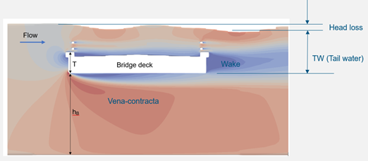
Figure 2.9: 2D CFD modelling of deck and rail bridge

Numerous 2D CFD models indicated that a generalised form for loss coefficient vs downstream water level above the soffit of the deck, TW, was possible, shown in Figure 2.10 for the case where the under-deck height to bed, h_b, was 4 times the deck thickness, T.

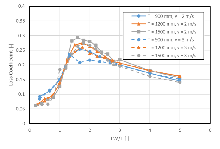
Figure 2.10: Generalised loss coefficient from 2D CFD modelling of bridge deck and rails

A full-scale bridge was gauged and the afflux recorded during a significant overtopping event in February 2022. 3D CFD models of the same bridge and surrounds were run, with reasonable agreement as shown in Figure 2.11. Further, the shape of the results appears very similar to that of the generalised 2D results shown in Figure 2.10.

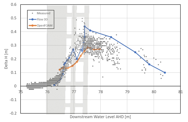
Figure 2.11: Full scale afflux measurements and 3D CFD model results for deck and rail bridge

A layered loss model was implemented in TUFLOW HPC as per Section 2.4.2, and a 2D HPC model of the bridge and surrounds was run. The results, shown in Figure 2.12, were in excellent agreement with the measured data.

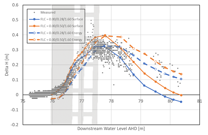
Figure 2.12: TUFLOW HPC afflux results for deck and rail bridge using new 2d_bg layer

2.4.2 New Input Layer for Modelling Bridge Structure in 2D

The 2023-03 Release introduces the new BG Shape input layer (2d_bg) to set up bridge structures in 2D domain. The new input layer is read in using the .tgc command “Read GIS BG Shape ==”. The new method is similar to the Method D layered flow constriction approach introduced in the 2020‑10 Release (Section 3.4.2 of the 2020 Release Notes), with the GIS layer attributes tidied up for easier user input. The three layers are now called the “pier layer”, the “deck layer” and the “rail layer” for clarity. The new attributes are:

• ID = Unique bridge ID.
• Option = Reserved for future use.
• Pier_pBlockage = The percentage blockage of the pier Layer. For example, enter ‘5’ for a blockage of 5%.
• Pier_FLC = Pier layer form loss coefficient.
• Deck_Soffit = The elevation of the bridge soffit (m or ft).
• Deck_Depth = The thickness of the bridge deck (m or ft).
• Deck_Width = The bridge width in the predominant direction of flow (m or ft).
• Deck_pBlockage = The percentage blockage of the deck layer. Enter ‘100’ for a solid bridge deck obstruction.
• Rail_Depth = The depth of the rail layer (m or ft).
• Rail_pBlockage: The percentage blockage of the rail layer.
• SuperS_FLC: The combined form loss coefficient for the deck and the rail layers. Two layers are treated as a single “super structure” layer in this new bridge method.
• SuperS_IPf: A factor to set the elevation of the inflection point (IP) at which the transition from pressure flow to drowned flow commences. The default value is 1.6.

• Cf: A calibration factor used to adjust the automatically generated FLC (default = 1.0). See Section 2.4.3.

The 2d_bg layer adjusts the FLC value in the vertical as follows: \[\begin{equation} {FLC}_{total} = \left( {FLC}_{pier} + {FLC}_{SuperS}\frac{y_{SuperS}}{D_{IP}} \right)\frac{(y_{pier} + y_{SuperS})}{y_{total}} \tag{2.7} \end{equation}\]

With: \[\begin{equation} y_{SuperS,max} = D_{IP} \tag{2.8} \end{equation}\]

\[\begin{equation} y_{pier,max} = D_{peir} \tag{2.9} \end{equation}\]

Where:

• \(y_{SuperS}\) = Depth of water above the bridge soffit in the super structure layer.
• \(D_{IP}\) = Depth to the inflection point from the bridge soffit.
• \(y_{pier}\) = Depth of water in the pier layer.
• \(D_{peir}\) = Depth to the pier layer, i.e. the vertical distance from the bed level to the bridge soffit.
• \(y_{total}\) = Total depth of water from the bed to the water surface level

The vertical distribution of the form loss coefficient has the following characteristics:

• Water level below the deck layer: The same result as the 2d_lfcsh approaches, i.e. a constant form loss based on that specified for the pier layer (\({FLC}_{pier}\)) is applied.
• Water level between the deck soffit and the inflection point: The FLC value is linearly increased from \({FLC}_{pier}\) to \({FLC}_{pier}\) + \({FLC}_{SuperS}\) (the combined form loss coefficient for the superstructure layer). The observations from the CFD and the field measurement indicate the inflection point is located around 1.6 times the bridge deck depth (\(D_{Deck}\)) above the bridge soffit. The “Inflection Depth” (\(D_{IP}\)) is assumed as:

\[\begin{equation} D_{IP} = SuperS_{IPf}\left( D_{Deck}{Blockage}_{Deck} + D_{Rail}{Blockage}_{Rail} \right) \tag{2.10} \end{equation}\]

• Note that the effect of partial blockage at the rail layer is considered by adding the rail layer depth (\(D_{Rail}\)) to the inflection depth proportionally based on the rail layer blockage (\({Blockage}_{Rail}\)).

• Above the inflection point the FLC gradually reduces with increasing depth (in a similar manner to the 2D Layered Flow Constrictions PORTION and METHOD C approaches), shown in Figure 2.13. This is to simulate the transition to drowned flow and tendency to zero energy losses with increasing depth over the bridge deck.

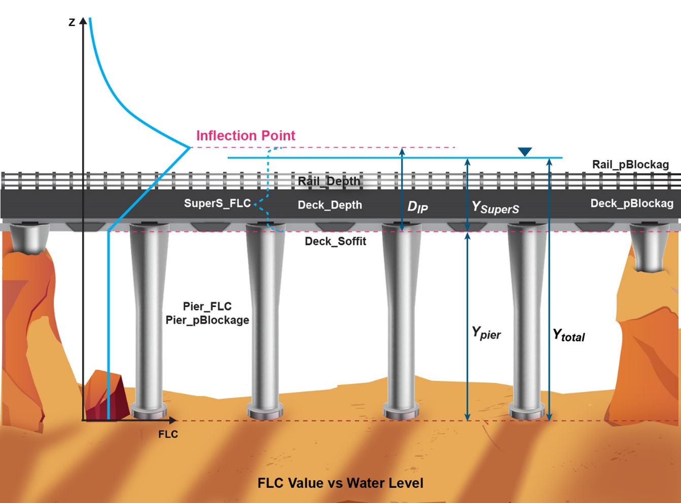
Figure 2.13: 2D BG Shape Attributes and Vertical Distribution of Form Loss Coefficient

In addition to the above method, build 2023-03-AD introduces three more methods to calculate the depth averaged FLC:

BG FLC Default Approach == [ {LINEAR} | LINEAR-CONSTANT | PARABOLIC | INVERTED-PARABOLIC ]

• LINEAR: the default option introduced above. The depth averaged FLC value is linearly increased from the bottom of the bridge deck to the inflection point. After the inflection point it gradually reduces.

• LINEAR-CONSTANT: the depth averaged FLC is linearly increased from the bottom of the bridge deck to the top of the bridge deck. Between the top of the bridge deck and the inflection point, the FLC is kept constant. After the inflection point it gradually reduces.

• PARABOLIC: the depth averaged FLC is increased using a parabolic function from the bottom of the bridge deck to the inflection point. After the inflection point it gradually reduces.

• INVERTED-PARABOLIC: the depth averaged FLC is increased using an inverted parabolic function from the bottom of the bridge deck to the inflection point. After the inflection point it gradually reduces.

The vertical profiles of the depth averaged FLC values applied by the four methods are illustrated in the Figure 2.14.

Figure 2.14: Depth averaged FLC applied by 4 bridge FLC approaches

Other key features of the BG layer are:

• The BG layer does not apply geometry updates. This not only offers simplicity, but also is a desirable option considering that the size of TIN polygons used to modify the bridge bed elevations are often different from the size of polygon used to select BG cell faces.
• For a line layer a “Deck_Width” value of zero sets the layer as a thin line. It selects one row of faces in the direction of flow, and the FLC value is applied to the faces unchanged. A “Deck_Width” value larger than zero sets the layer as a thick line that selects a whole cell, i.e. two faces in the direction of flow. The FLC values at the faces are divided by two. The wide line feature is not supported by the BG layer. Note, BG polygon shapes are recommended if more than 3 rows of faces must be selected.
• For a polygon layer, the “Deck_Width” defines the bridge width in the predominant direction of flow. This value is used to distribute the total FLC value to the selected faces, i.e.:
  \[\begin{equation} {FLC}_{face} = \frac{FLC} {Deck\_Width} * Cell\ Size \tag{2.11} \end{equation}\]

This means users no longer need to convert the FLC value to “form loss per metre”, which is required by the 2D Layered Flow Constrictions polygons.

Note: Build 2023-03-AB caps “Cell Size / Deck_Width” at 1. Previously, a face FLC larger than the original FLC was incorrectly applied when the model cell size is larger than the Deck_Width defined.

The point only layer (2d_bg_pts) is also supported. This layer can be used to spatially vary the bridge soffit, the deck depth, and the rail depth. The attributes for this layer include:

• Deck_Soffit = The elevation of the bridge soffit (m or ft).
• Deck_Depth = The thickness of the bridge deck (m or ft).
• Rail_Depth = The depth of the rail layer (m or ft).
• R1 ~ R3: Reserved for future use.

2.4.3 Automatic Generation of Superstructure FLC

Build 2023-03-AC implemented a new feature to automatically generate the superstructure FLC value based on the CFD benchmarking study (Collecutt et al., 2022). This feature has been further developed in build 2023-03-AD.

Blank BG FLC Approach == [ {NONE} | METHOD A | METHOD B ]

• NONE: the default approach, i.e. Superstructure FLC must be specified manually.

• METHOD A: The blank superstructure FLC values will be calculated based on the ratio of the depth of the pier layer (\(D_{Pier}\) in the equations above) and the thickness of the super structure layer:

\[\begin{equation} T_{SuperS} = D_{Deck}{Blockage}_{Deck} + D_{Rail}{Blockage}_{Rail} \tag{2.12} \end{equation}\]

Build 2023-03-AD fixed a bug where ‘SuperS_IPf’ was used in the calculation of \(T_{SuperS}\).

• METHOD B: The blank superstructure FLC values will be calculated based on the ratio of the depth of the pier layer (\(D_{Pier}\)) and the thickness of the deck layer:

\[\begin{equation} T_{SuperS} = D_{Deck}{Blockage}_{Deck} \tag{2.13} \end{equation}\]

With Method A and B, the superstructure FLC value is linearly interpolated within the \(D_{Pier}\)/\(T_{SuperS}\) range of 1~10 and capped at 0.6 and 0.16 outside this range, as shown in the Figure 2.15.

Figure 2.15: CFD benchmarking study of FLC vs \(D_{Pier}\)/\(T_{SuperS}\) ratio (\(h_{B}\)/\(T\) in the original paper)

Build 2023-03-AD introduces a calibration factor (the 2d_bg ‘Cf’ attribute) that is applied as a multiplier to the automatically generated superstructure FLC.

2.4.4 Grouped Structure Output

The new 2d_bg layer can be used with 2D plot output structure group outputs (2d_po ‘QS’ type) in the same manner as the 2D Layered FC Shape input (2d_lfcsh).

2.5 Advection Dispersion

2.5.1 HPC Support for Multiple Constituents Per Simulation

When using the HPC solver it is now possible to run up to 20 advection-dispersion constituents in a single simulation. This is the same limit as when running advection-dispersion with the Classic solver. Prior to the 2023-03 Release if running advection-dispersion with HPC only a single constituent could be modelled.

Advection-dispersion is currently not supported in the Quadtree module.

2.5.2 HPC Support for Constituent Settling and Decay

For the 2023-03 Release the HPC solver supports the ability to model constituent settling and/or decay. This functionality is detailed in Section 4.6 of the TUFLOW AD Manual.

2.5.3 Layered Interflow - Advection Dispersion TGC Commands

Initial concentrations can be set within the groundwater layers using the following .tgc commands (note, not done in the AD Control File):

[Set | Read GIS | Read GRID] IGW Conc Layer N1,N2,..N Tracer M1,M2,..M == [value | /path/to/file]

Where:

• N = The groundwater layer number (able to reference multiple in a single command)
• M = The tracer number (able to reference multiple in a single command) as ordered in the AD Global Database

If a layer number is not referenced, it is assumed to apply to layer 1. Likewise, if a tracer number is not referenced it is assumed to apply to the first tracer. Note, the order that ‘Layer’ and ‘Tracer’ appear in the command does not matter (i.e. tracer numbers could be listed before layer numbers).

2.6 Non-Newtonian Mixing

Non-Newtonian viscosity formulation was introduced, for a uniform fluid, in the 2020-01-AA Release. This has now been extended to consider mixing of the non-Newtonian fluid with water. To implement this, a passive tracer must be included in the model, requiring a license for the advection-dispersion (AD) module. The AD setup is the same as detailed in the TUFLOW AD Manual. More than one tracer field is permissible, but the non-Newtonian mixing module will assume that the first tracer represents the fraction of non-Newtonian fluid, in the range 0 to 1. Care must be taken to ensure that boundary data and initialisation commands strictly adhere to this range. Where the tracer value is 1, the properties of the fluid will be exactly the non-Newtonian properties as specified with Viscosity Coefficients command. For tracer values between 0 and 1, the non-Newtonian properties are transitioned using power-law equations for the three variables in the Hershel-Bulkley equation.

\[\begin{equation} \xi = a^{m} \tag{2.14} \end{equation}\] \[\begin{equation} \rho' = (1 - a)\rho_{w} + a\rho_{NN} \tag{2.15} \end{equation}\] \[\begin{equation} K' = (1 - a^{m})\nu_{w} + a^{m} K_{NN} \tag{2.16} \end{equation}\] \[\begin{equation} n' = (1 - a^{o})1.0 + a^{o} n_{NN} \tag{2.17} \end{equation}\] \[\begin{equation} \tau_{0}' = a^{p}\tau_{0,NN} \tag{2.18} \end{equation}\]

Where:

• \(a\) = the tracer value (0~1)
• \(m\) = the non-Newtonian mixing exponent for the viscosity parameter
• \(o\) = the non-Newtonian mixing exponent for the power law parameter
• \(p\) = the non-Newtonian mixing exponent for the yield stress
• \(\rho\) = density of fluid (kg/m³)
• \(\nu\) = kinematic viscosity (m²/s)
• \(K\) = the Hershel-Bulkley viscosity parameter (Pa sⁿ)
• \(n\) = the Hershel-Bulkley power law exponent
• \(\tau_{0}\) = the material yield stress (Pa)

and subscripts \(w\) denotes water, \(NN\) denotes pure non-Newtonian fluid.

In the 2023-03-AA and 2023-03-AB builds, only one non-Newtonian mixing exponent was allowed for. The 2023-03-AC build allows for three mixing exponents m, o, p, to be specified. Alternative, if only one mixing exponent is specified, that value is used for all three exponents.

The bed fraction and 2D viscosity are computed using the non-Newtonian method with the blended parameters The bed friction is then limited to be no less than that predicted from Manning’s equation, and the 2D viscosity is limited to be no less that that predicted from the Wu viscosity formulation with 3D and 2D coefficients of 7 and 0 respectively.

To utilise non-Newtonian mixing in a model, the following is required:

1. Select the non-Newtonian viscosity formulation and specify the coefficients for pure non-Newtonian fluid:

   Viscosity Formulation == Non-Newtonian

   Viscosity Coefficients == k, n, muLow, muHigh, tau0

2. Include a passive tracer as per standard AD setup (refer to the TUFLOW AD Manual), making sure boundary data and initialisation are scaled in range 0 to 1.

3. Specify the mixing exponents, m, o, and p to be used:

   Non-Newtonian Mixing Exponent == <float> | {0} ! used for all three of m, o, p exponents

   Non-Newtonian Mixing Exponent == <float>, <float>, <float> | {0, 0, 0} ! m, o, p exponents

Note that if the non-Newtonian mixing exponent is not specified it defaults to zero which turns the mixing formulation off, and all fluid in the model will be treated as non-Newtonian regardless of tracer value.

2.7 Minor Enhancements and Bug Fixes

2.7.1 Fix to Memory Efficient Quadtree Meshing Algorithm

The 2023-03 Release fixes a bug that could occur when using the .qcf command:

Quadtree Mesh Processing Method == Memory Efficient

Previously, when there were barely overlapping hidden domains (generated as part of the meshing algorithm) that only just overlapped by one or two cells in the top left corner, sometimes the order of the domains would cause cells to be deactivated incorrectly. This would cause holes in the final generated quadtree mesh.

2.7.2 Duplicate Material IDs

When reading in materials files, in either .tmf or .csv, the 2023-03 Release handles duplicate material IDs differently. For the 2023-03 Release duplicate material IDs will now override previous values. This includes if the material ID is contained in the same material file or different material file. Overwriting duplicate data is more consistent with other processing in TUFLOW.

WARNING 2564 is issued each time a duplicate ID is encountered. Previously if a duplicate material ID was found, it would be discarded with WARNING 2481.

2.7.3 Duplicate Soil IDs

Similar to the duplicate material ID change above, when reading soils files (.tsoilf) duplicate soil IDs will now override previous values in the 2023-03 Release. This includes if the soil ID is contained in the same soil file or different soil file. Overwriting duplicate data is more consistent with other processing in TUFLOW.

WARNING 2500 is issued each time a duplicate ID is encountered.

2.7.4 Check Added for Valid Non-Newtonian Coefficients

A check has been added if Non-Newtonian formulation has been specified without valid Non-Newtonian coefficients. For build 2023-03-AA onwards ERROR 2572 will be generated if no or invalid coefficients have been specified.

2.7.5 ERROR Message for Overlapping Layered Flow Constriction Shape and 2D Bridge Shape

Build 2023-03-AA produces ERROR 2467 when an overlapping Layered Flow Constriction Shape or 2D Bridge Shape is detected. Previously, all the duplicated Layered Flow Constriction Shapes have been processed during the cell side form loss calculation. For TUFLOW Classic, the last read Layered Flow Constriction Shape would be used. However, for TUFLOW HPC, the order to process the Layered Flow Constriction Shapes could not be determined due to the nature of GPU parallel computing. This mean there is no way to check which value was applied in the hydraulic calculation.

2.8 2023-03-AB Minor Enhancements and Bug Fixes

2.8.1 Bug Fix to HR Breakline Adjustment with Output Zone

Build 2023-03-AB fixes a memory allocation issue when “HR Thin Z Line Output Adjustment == ON ALIGNMENT” are used in conjunction with Output Zones. Previously, this could cause the simulation to crash without error.

2.8.2 Read GIS / GRID Soil Layer Accepts Multiple Layer Numbers

Build 2023-03-AB accepts multiple layer numbers in the GIS / GRID command within the TGC, e.g:

Read GIS Soil Layer 1, 2 == gis\2d_soil_001.gpkg

2.8.3 Un-Deprecated GWD and GWL Commands

Build 2023-03-AB un-deprecates the GWD (groundwater depth) and GWL (groundwater level) commands in the TGC which were originally deprecated in favour of the newer “Soil Thickness” and “Soil Base Elevation” commands. However, to conserve backward compatibility, these commands have been un-deprecated when not using the interflow functionality.

2.8.4 Bug Fix HPC GWQ PO Units

Build 2023-03-AB fixes the units output from HPC for groundwater flow (line) which was reporting in mm³/s rather than m³/s. Quadtree was correctly reporting in m³/s.

2.8.5 Bug Fix for Ground Water Outputs

Build 2023-03-AB fixes an issue which would cause advection-dispersion outputs to be written for groundwater layers if advection-dispersion was being modelled without soils.

2.8.6 Bug Fix for Infiltration Outputs in Classic

Build 2023-03-AB fixes an issue where infiltration outputs (CI and IR) were being suppressed when running TUFLOW Classic. For the 2023-03-AA Build, WARNING 2587 was issued and these data types not output. This did not affect the infiltration computations.

2.8.7 Bug Fix for HPC Breakline Memory Release

Build 2023-03-AB correctly releases memory when running TUFLOW HPC at the end of the simulation. Previously when running multiple simulations through an external 1D engine, ERROR 3544 could be generated on the second simulation.

2.8.8 Infiltration When No Soil Capacity and Infinite Depth Soil

When a soil has an initial moisture fraction greater than the soil porosity (i.e. the soil capacity is zero) TUFLOW issues WARNING 2508. For builds prior to 2023-03-AB, when no soil thickness or soil base elevation is specified (i.e. soil thickness is infinite) and the soil capacity is zero, infiltration occurs despite WARNING 2508 being generated. For build 2023-03-AB this has been fixed so that no infiltration occurs – consistent with the warning message.

2.9 2023-03-AC Minor Enhancements and Bug Fixes

2.9.1 Bug Fix to Default SGS Elevation

Build 2023-03-AC fixes an issue that occurred, when using SGS, where the bed elevation defaulted to 0 m if the Set Zpts command was not used. This meant the error message “ERROR 2206 - ZH value not initialised (exceeds 99998 m)” was not triggered correctly. Build 2023-03-AC now sets the default elevation as 99999 m, consistent with non-SGS models.

This could also cause the final SGS elevations to be re-processed after each model initialisation, in this case CHECK 3551 was issued.

2.9.2 Bug Fix to Quadtree Clip Region

Build 2023-03-AC fixes an issue where, if using multiple clip regions with the Read GRID Zpts command, they could be ignored. This issue could occur if some of the clip regions were located outside of the model domain, or the quadtree sub-domain(s), the entire clip region file was ignored.

Build 2023-03-AC only skips those clip regions outside the model domain, and still applies the clip regions located inside the model domain.

2.9.3 Bug Fix to Read TIN Command in HPC Model

Build 2023-03-AC fixes an issue that TIN Angles command wasn’t read before the TINs were created in HPC models. This could cause inconsistency between the TINs created by Classic and HPC models.

Build 2023-03-AD extends this fix to HPC models with quadtree refinement.

2.9.4 Bug Fix Quadtree 2d_zsh Snapped to Code

Build 2023-03-AC fixes an issue that could cause TUFLOW to exit uncleanly. This was caused when a 2d_zsh (or similar e.g. 2d_lfcsh) was snapped along the 2d_code polygon. This bug only affected Quadtree models.

2.9.5 Bug Fix for “Blockage Return Period” Command

Prior to Build 2023-03-AC, the “Blockage Return Period == AEP” command is not applied if it’s read after the Blockage Matrix File command. The first column in the matrix file is still treated as “ARI”. Build 2023-03-AC fixes this issue and the “Blockage Return Period == AEP” command can be specified either before or after the Blockage Matrix File command.

2.9.6 Bug Fix for Long Breaklines in Quadtree

Prior to Build 2023-03-AC, a long breakline in quadtree model could cause stack overflow issue if it selects more than 10,000 cells. Build 2023-03-AC adds a “ERROR 2859 - Number of quadtree cells selected by a polyline exceeds the limit of 10000” message. If this error is encountered, it is recommended to split the long breakline in to shorter sections.

2.10 2023-03-AD Minor Enhancements and Bug Fixes

2.10.1 Bug Fix HPC Initial Tracer Concentration

Build 2023-03-AD fixes a tracer concentration initialisation issue for the HPC Advection-Dispersion module. Previously, the initial tracer concentrations were all set as zero.

2.10.2 Bug Fix for Auto Generated Bridge FLC with ‘Bridge_width’

Build 2023-03-AD fixes an issue where the 2d_bg ‘deck_width’ attribute was not correctly applied to distribute the automatically calculated FLC (Section 2.4.3) to cell faces.

2.10.3 Bug Fix for Longitudinal Profile Output (LP) in Quadtree Models

Build 2023-03-AD fixes an issue where the Longitudinal Profile Output (Read GIS LP) could cause memory access violation in Quadtree models. A known issue caused by this memory access violation includes a change to inflow values from a QT boundary.

2.10.4 Bug Fix for Invalid 2d_code Values

Build 2023-03-AD introduces stricter checks when reading Code values specified with either the Set Code or Read GIS Code command in the .tgc. Valid options for cell code are:

• Code -1, inactive cell but included in outputs (HPC and Classic only)
  
• Code 0, inactive cell
  
• Code 1, active cell

Previously, values outside this range could be specified and this code would be included in the grid outputs. For the 2023-03-AD build any values >1 are treated as 1 and a values less than -1 are treated as -1. In both cases WARNING 2905 is output.

Note, code values of 2 are output in the _grd check file for cells assigned as boundary cells, and this happens automatically.

2.10.5 Bug Fix for Large SX/HX BC Connections in Quadtree

Build 2023-03-AD fixes a stack overflow issue in quadtree models that could occur if a SX/HX connection selects a large number of cells. Prior to Build 2023-03-AD, this could cause the model to crash without error message.

References

Collecutt, G., Baeumer, U., Gao, S., & Syme, W. (2022). Bridge Deck Afflux Modelling – Benchmarking of CFD and SWE Codes to Real-World Data. Hydrology & Water Resources Symposium. https://tuflow.com/media/7554/2022-bridge-deck-afflux-modelling-benchmarking-of-cfd-and-swe-codes-to-real-world-data-collecutt-et-al-hwrs.pdf